The tutorial explains how to use COUNTIFS and COUNTIF formulas with multiple criteria in Excel based on AND as well as OR logic. You will find a number of examples for different data types - numbers, dates, text, wildcard characters, non-blank cells and more.
Of all Excel functions, COUNTIFS and COUNTIF are probably most often mixed up because they look very much alike and both are purposed for counting cells based on the specified criteria.
The difference is that COUNTIF is designed for counting cells with a single condition in one range, whereas COUNTIFS can evaluate different criteria in the same or in different ranges. The aim of this tutorial is to demonstrate different approaches and help you choose the most efficient formula for each particular task.
Excel COUNTIFS function - syntax and usage
The Excel COUNTIFS function counts cells across multiple ranges based on one or several conditions. The function is available in Excel 365, 2021, 2019, 2016, 2013, Excel 2010, and Excel 2007, so you can use the below examples in any Excel version.
COUNTIFS syntax
The syntax of the COUNTIFS function is as follows:
- criteria_range1 (required) - defines the first range to which the first condition (criteria1) shall be applied.
- criteria1 (required) - sets the condition in the form of a number, cell reference, text string, expression or another Excel function. The criteria defines which cells shall be counted and can be expressed as 10, "<=32", A6, "sweets".
- [criteria_range2, criteria2]… (optional) - these are additional ranges and their associated criteria. You can specify up to 127 range/criteria pairs in your formulas.
In fact, you don't have to remember the syntax of the COUNTIF function by heart. Microsoft Excel will display the function's arguments as soon as you start typing; the argument you are entering at the moment is highlighted in bold.

Excel COUNTIFS - things to remember!
- You can use the COUNTIFS function in Excel to count cells in a single range with a single condition as well as in multiple ranges with multiple conditions. If the latter, only those cells that meet all of the specified conditions are counted.
- Each additional range must have the same number of rows and columns as the first range (criteria_range1 argument).
- Both contiguous and non-contiguous ranges are allowed.
- If the criteria is a reference to an empty cell, the COUNTIFS function treats it as a zero value (0).
- You can use the wildcard characters in criteria - asterisk (*) and question mark (?). See this example for full details.
How to use COUNTIFS and COUNTIF with multiple criteria in Excel
Below you will find a number of formula examples that demonstrate how to use the COUNTIFS and COUNTIF functions in Excel to evaluate multiple conditions.
How to count cells with multiple criteria (AND logic)
This scenario is the easiest one, since the COUNTIFS function in Excel is designed to count only those cells for which all of the specified conditions are TRUE. We call it the AND logic, because Excel's AND function works this way.
Formula 1. COUNTIFS formula with multiple criteria
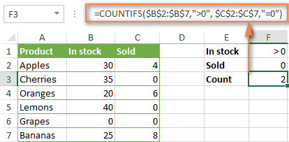
Suppose you have a product list like shown in the screenshot below. You want to get a count of items that are in stock (value in column B is greater than 0) but have not been sold yet (value is column C is equal to 0).
The task can be accomplished by using this formula:
=COUNTIFS(B2:B7,">0", C2:C7,"=0")
And the count is 2 ("Cherries" and "Lemons"):
Formula 2. COUNTIFS formula with two criteria
When you want to count items with identical criteria, you still need to supply each criteria_range / criteria pair individually.
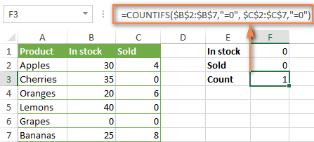
For example, here's the right formula to count items that have 0 both in column B and column C:
=COUNTIFS($B$2:$B$7,"=0", $C$2:$C$7,"=0")
This COUNTIFS formula returns 1 because only "Grapes" have "0" value in both columns.
Using a simpler formula with a single criteria_range like COUNTIFS(B2:C7,"=0") would yield a different result - the total count of cells in the range B2:C7 containing a zero (which is 4 in this example).
How to count cells with multiple criteria (OR logic)
As you have seen in the above examples, counting cells that meet all of the specified criteria is easy because the COUNTIFS function is designed to work this way.
But what if you want to count cells for which at least one of the specified conditions is TRUE, i.e. based on the OR logic? Overall, there are two ways to do this - by adding up several COUNTIF formulas or using a SUM COUNTIFS formula with an array constant.
Formula 1. Add up two or more COUNTIF or COUNITFS formulas
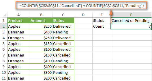
In the table below, supposing you want to count orders with the "Cancelled" and "Pending" status. To have it doen, you can simply write 2 regular Countif formulas and add up the results:
=COUNTIF($C$2:$C$11,"Cancelled") + COUNTIF($C$2:$C$11,"Pending")
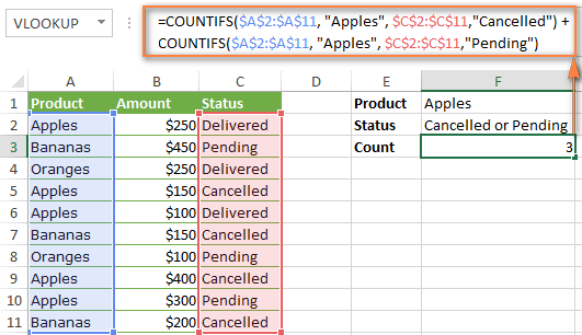
In case each of the functions is supposed to evaluate more than one condition, use COUNTIFS instead of COUNTIF. For example, to get the count of "Cancelled" and "Pending" orders for "Apples" use this formula:
=COUNTIFS($A$2:$A$11, "Apples", $C$2:$C$11,"Cancelled") + COUNTIFS($A$2:$A$11, "Apples", $C$2:$C$11,"Pending")
Formula 2. SUM COUNTIFS with an array constant
In situations when you have to evaluate a lot of criteria, the above approach is not the best way to go because your formula would grow too big in size. To perform the same calculations in a more compact formula, list all of your criteria in an array constant, and supply that array to the criteria argument of the COUNTIFS function. To get the total count, embed COUNTIFS inside the SUM function, like this:
In our sample table, to count orders with the status "Cancelled" or "Pending" or "In transit", the formula would go as follows:
=SUM(COUNTIFS($C$2:$C$11, {"cancelled", "pending", "in transit"}))
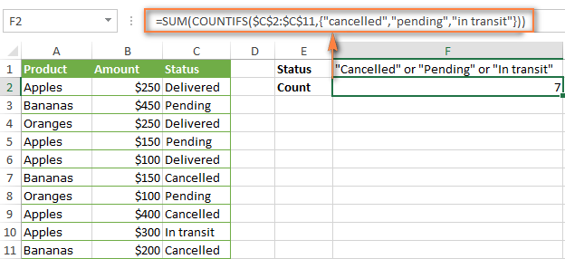
In a similar manner, you can count cells based on two or more criteria_range / criteria pairs. For instance, to get the number of "Apples" orders that are "Cancelled" or "Pending" or "In transit", use this formula:
=SUM(COUNTIFS($A$2:$A$11,"apples",$C$2:$C$11,{"cancelled","pending","in transit"}))

You can find a few more ways to count cells with OR logic in this tutorial: Excel COUNTIF and COUNTIFS with OR conditions.
How to count numbers between 2 specified numbers
By and large, COUNTIFS formulas for numbers fall into 2 categories - based on several conditions (explained in the above examples) and between the two values you specify. The latter can be accomplished in two ways - by using the COUNTIFS function or by subtracting one COUNTIF from another.
Formula 1. COUNTIFS to count cells between two numbers
To find out how many numbers between 5 and 10 (not including 5 and 10) are contained in cells C2 through C10, use this formula:
=COUNTIFS(C2:C10,">5", C2:C10,"<10")
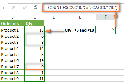
To include 5 and 10 in the count, use the "greater than or equal to" and "less than or equal to" operators:
=COUNTIFS(B2:B10,">=5", B2:B10,"<=10")
Formula 2. COUNTIF formulas to count numbers between X and Y
The same result can be achieved by subtracting one Countif formula from another. The first one counts how many numbers are greater than the lower bound value (5 in this example). The second formula returns the count of numbers that are greater than the upper bound value (10 in this case). The difference between the first and second number is the result you are looking for.
- =COUNTIF(C2:C10,">5")-COUNTIF(C2:C10,">=10") - counts how many numbers greater than 5 and less than 10 are in the range C2:C10. This formula will return the same count as shown in the screenshot above.
- =COUNTIF(C2:C10, ">=5")-COUNTIF(C2:C10, ">10") - the formula counts how many numbers between 5 and 10 are in the range C2:C10, including 5 and 10.
How to use cell references in COUNTIFS formulas
When using logical operators such as ">", "<", "<=" or ">=" together with cell references in your Excel COUNTIFS formulas, remember to enclose the operator in "double quotes" and
add an ampersand (&) before a cell reference to construct a text string.
In a sample dataset below, let's count "Apples" orders with amount greater than $200. With criteria_range1 in cells A2:A11 and criteria_range2 in B2:B11, you can use this formula:
=COUNTIFS($A$2:$A$11, "Apples", $B$2:$B$11, ">200")
Or, you can input your criteria values in certain cells, say F1 and F2, and reference those cells in your formula:
=COUNTIFS($A$2:$A$11, $F$1, $B$2:$B$11, ">"&$F$2)
Please notice the use of absolute cell references both in the criteria and criteria_range arguments, which prevents the formula from being broken when copied to other cells.
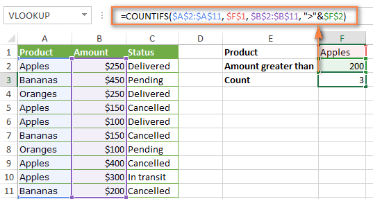
For more information about the use of an ampersand in COUNTIF and COUNTIFS formulas, please see Excel COUNTIF - frequently asked questions.
How to use COUNTIFS with wildcard characters
In Excel COUNTIFS formulas, you can use the following wildcard characters:
- Question mark (?) - matches any single character, use it to count cells starting and/or ending with certain characters.
- Asterisk (*) - matches any sequence of characters, you use it to count cells containing a specified word or a character(s) as part of the cell's contents.
Tip. If you want to count cells with an actual question mark or asterisk, type a tilde (~) before an asterisk or question mark.
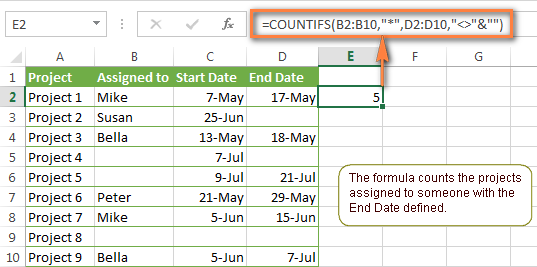
Now let's see how you can use a wildcard char in real-life COUNTIFS formulas in Excel. Suppose, you have a list of projects in column A. You wish to know how many projects are already assigned to someone, i.e. have any name in column B. And because we are learning how to use the COUNTIFS function with multiple criteria, let's add a second condition - the End Date in column D should also be set.
Here is the formula that works a treat:
=COUNTIFS(B2:B10,"*",D2:D10,"<>"&""))
Please note, you cannot use a wildcard character in the 2nd criteria because you have dates rather that text values in column D. That is why, you use the criteria that finds non-blank cells: "<>"&""
COUNTIFS and COUNTIF with multiple criteria for dates
The COUNTIFS and COUNTIF formulas you use for dates are very much similar to the above formulas for numbers.
Example 1. Count dates in a specific date range
To count the dates that fall in a certain date range, you can also use either a COUNTIFS formula with two criteria or a combination of two COUNTIF functions.
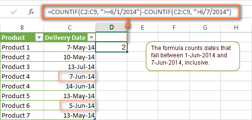
For example, the following formulas count the number of dates in cells C2 through C10 that fall between 1-Jun-2014 and 7-Jun-2014, inclusive:
=COUNTIFS(C2:C9, ">=6/1/2014", C2:C9, "<=6/7/2014")
=COUNTIF(C2:C9, ">=6/1/2014") - COUNTIF(C2:C9, ">6/7/2014")
Example 2. Count dates with multiple conditions
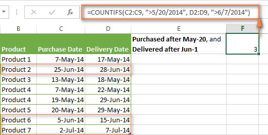
In the same manner, you can use a COUNTIFS formula to count the number of dates in different columns that meet 2 or more conditions. For instance, the below formula will find out how many products were purchased after the 20th of May and delivered after the 1st of June:
=COUNTIFS(C2:C9, ">5/1/2014", D2:D9, ">6/7/2014")
Example 3. Count dates with multiple conditions based on the current date
You can use Excel's TODAY() function in combination with COUNTIF to count dates based on the current date.
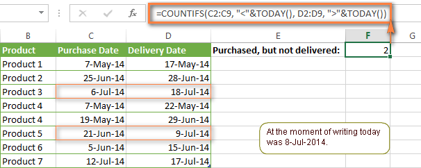
For example, the following COUNTIF formula with two ranges and two criteria will tell you how many products have already been purchased but not delivered yet.
=COUNTIFS(C2:C9, "<"&TODAY(), D2:D9, ">"&TODAY())
This formula allows for many possible variations. For instance, you can tweak it to count how many products were purchased more than a week ago and are not delivered yet:
=COUNTIFS(C2:C9, "<="&TODAY()-7, D2:D9, ">"&TODAY())
This is how you count cells with multiple criteria in Excel. I hope you will find these examples helpful. Anyway, I thank you for reading and hope to see you on our blog next week!
 by
by
1981 comments
Hi, I am trying to count the number of times a two separate strings of text appear in a column that also fall between two dates. I can get it to work if only looking for one string of text but am unsure how to look for two or more.
For example in my 'D' column I am looking for the number of times the text 'S05' appears if it falls between the dates 01/04/2019 and 01/04/2020 in column 'F'. The formula I currently have for this is:
=COUNTIFS($D$10:$D$32981,"S05*",$F$10:$F$32981,">=01/04/2019",$F$10:$F$32981,"<01/04/2020")
This works but I'd also like it to count the number of times the text 'HINGED5' appears in column 'D' at the same time. Are you able to assist?
Hello!
If you want to use OR logic, try this formula
=COUNTIFS($D$10:$D$32981,"S05*",$F$10:$F$32981,">=01/04/2019",$F$10:$F$32981,"<01/04/2020") + COUNTIFS($D$10:$D$32981,"*HINGED5*",$F$10:$F$32981,">=01/04/2019",$F$10:$F$32981,"<01/04/2020")
If you want to use AND logic, try this formula
COUNTIFS($D$10:$D$32981,"S05*", $D$10:$D$32981,"*HINGED5*", $F$10:$F$32981,">=01/04/2019",$F$10:$F$32981,"<01/04/2020")
This is described in the article above.
Thank you. I did try that formula after reading the article the first time but couldn't get it to work so I must have mistyped something. This is working perfectly for me know, much appreciated.
Hi, I need to work out a formula for the following:
I have 5 rows with different info...
A1 = date, A2 = name, A3 = description, A4 = shop, A5 = amount.
Now I have to add the total spent for each name and for different expenses.
For instance, Sam has spent P500 on employment cost, P200 on production cost and P3000 on capital investment
Sarah has spent P1000 on employment cost, P200 on production cost and P3000 on capital investment.
Now I have to calculate only employment cost and production cost for Sarah and then seperately for Sam as well.
How do I go about? Please help.....
Regards
Hi!
Use the SUMIFS function. Here is the article that may be helpful to you: Excel SUMIFS and SUMIF with multiple criteria
I hope this will help.
I am trying to count cell-specific values using "in-cell dropdown". I am able to count each of these using the "countif" formula, but how can I assign a value to each. An example would be I have "green" with cell values of .5, 4, 1 & 8.5 and "yellow" with values of 1, 10 & 3.5. How can I add all of these numbers together, for each of the different in-cell options?
I hope this makes sense. I have a good basic knowledge of excel and have been trying to learn more.
Thank you!
Hello!
You can sum only values written in a cell. You cannot sum possible values from the drop-down list, since this is a formula.
Hello, i want to know if there is a formula that picks up first Column A is filled but Column B & C are Blank?
Thank you
Hi, I am trying to use the COUNTIFS function as below...
Column A "start date", I want it to count all dates before 01/04/2021 but then also count in Column B "end date" all dates after 01/04/2021, there are 5 in my test sheet but it's only pulling two when I use this formula =COUNTIFS(Participants!A:A, ""&"1/4/2021")
I need it to first count those who started before 1st April 2021 then out of those how many finished after 1st April 2021 - please help!
Hello!
If I understand your task correctly, the following formula should work for you:
=COUNTIFS(A1:A6,">"&"1/4/2021",B1:B6,"<"&"1/4/2021")
If this is not what you wanted, please describe the problem in more detail.
Hi!
Sorry the full formula didn't paste correctly in my first comment, the one you have suggested is the formula I have tried but for some reason it is only pulling 2 of the 5 entries that it should. I'm not sure where I'm going wrong. Thanks
Hi!
I can't see your details. Therefore my formula cannot work 100%. Change it for your data.
Hi
Novice here looking for help!
I’m looking to add up the total volume in column A of attributes in column B but only if column C contains the word scan.
A B C D
4 Apples Scan 1 Jan
4 Pears Scan 2 Feb
2 Apples 9 Feb
2 Apples Scan 17 March
1 Scan 21 March
So I’d end up with:
Apples = 6
Pears = 4
I also need the formulae to work if the table has been filtered. I have a column D with a date in it so if I filter the data to just show January dates for example it would have Apples = 4, Pear = 0.
Hope that all makes sense!
Thanks
Dave
Hello!
I believe the following formula will help you solve your task:
=SUMIFS(A1:A4,B1:B4,"apples",C1:C4,"scan")
I recommend reading this guide: Excel SUMIFS and SUMIF with multiple criteria and Excel SUMIFS date range formula - sum if between two dates
I hope I answered your question. If something is still unclear, please feel free to ask.
Hi - I am trying to create a COUNTIFS to give me a total count based on 5 criteria to be satisfied. 2 of my criteria includes counting how many rows have a value <0.1% , however the formula isnt working. It works however when i use a range 0.1%-1% for example. Is this because of the signs?
Hi!
Please specify which formula you mean and describe the problem in more detail
Hi Team,
My Question is the expected result count = 3 which is not coming with below Query.
=SUM(COUNTIFS($A2:$A11,{"Apples",Bananas"},$C2:$C11,{"Delivered","Pending"}))
Hello!
Pay attention to the following paragraph of the article above — How to count cells with multiple criteria (OR logic)
Hi,
I have a spreadsheet containing tasks and the percentage of completing each task, I am trying to get the number of tasks which 100% completed using function CountIFS as following
=COUNTIFS(B5:D47,"*leak test*",F5:F47,"=100%")
each time doing that I got error #VALUE! , So Could you Please Help, Note: leak test is a repeated task
thanks
Hello!
The ranges in which the COUNTIFS function checks for values must be the same size.
Change B5:D47 to B5:B47, C5:C47, В5:В47 .
Pay attention to the following paragraph of the article above — Count cells with multiple criteria (OR logic)
Good day! is it possible to count data in a single criteria with multiple data inputted in a cell?
Example:
Column 1: Gadget Ownership
Cell 1: Laptop, Desktop
Cell 2: Smartphone, Desktop
Hello!
I’m not sure I got you right since the description you provided is not entirely clear. However, it seems to me that the formula below will work for you:
=SUM(--ISNUMBER(SEARCH(D1,A1:A20,1)))
D1 - criteria
I have Yes/No in a column. I want to count all "No" till it encounters the first "Yes".Please help
Hello!
If the records in the column start at row 1, then try the formula
=MATCH("Yes",D1:D1000,0)-1
You can learn more about MATCH function in Excel in this article on our blog.
Hello Sir, first of thing, thank you very much for your help with a lot of information in your website, unfortunately, I am still having a problem. Could you help me please?
The formula to count and multiply that I am using is:
=((COUNTA(C5:E5;G5:I5;K5:M5;O5:Q5;S5:U5;W5))*4)+((COUNTA(B5;F5;J5;N5;R5;V5)*10))
However I want count only text values (GR, CH, IT, MI) and multiply by 4 and 10, and not the values (FER, GER). In the same cell I can setup all the values with menu row. If I set up the value FER or GER, the cell dont will be counted.
thanks in advanced.
Hello!
Please re-check the article above since it covers your task.
Hello Sir, I need help with the same kind of a situation. I have multiple criteria from the same column so i am using an array. I am using the below formula but seeing incorrect results.. please suggest an alternative. I will try to put it across as good as possible but please let me know if you need more information.
=SUM(COUNTIFS(CriteriaRange1,{criteria 1, criteria 2, criteria 3},CriteriaRange2,{criteria 4, criteria 5, criteria 6},CriteriaRange3,{criteria 7, criteria 8, criteria 9}))
Hi i need help with my table can you help me my table goes like this
Term Definition Function/formula
1 Adding
2 Subtracting
3 Multiple
4 Divide
5 Sum
6 Min
7 Max
8 Count
9 Counta
10 Average
11 Median
12 Concatenate
13 If
14 Countif
15 VLookup
Hi! I am trying to create the count if function with multiple criteria, but I cant seem to get it to work. This is for scoring a particular skill with a set score for each questions. I don't have any problems if the score is constant, but how about if I have 2 scores?
Hi Svetlana,
I am looking for a solution where I will search 3 values in one column like "cancelled" or "pending" or "in transit" and then pick the corresponding value in the product column in a list. So I want index with countif, if that makes sense to you. Because match can not find 3 values and then give me the corresponding values in the product column.
Regards,
Abrar
Hi,
I have a question - What formula do I use when I have column that shows OPEN (AR3 cell) and all the tally numbers below AR3 cell AR4 to AR122 to match for QTY on hand column (D3) for each P/N D4 thru D122. Next day the OPEN will move to AT3 cell and AR3 cell will be closed.
Hi,
I am trying to use countifs using a range. I would like to it to count items that meet the first 2 aspects ('Sheet1'!$C:$C,"PHASE",'Sheet1'!E:E,"CONTACT") but the third aspect I would like it to count a range.
For a single column in the 3rd aspect, this formula works:
COUNTIFS('Sheet1'!$C:$C,"PHASE",'Sheet1'!E:E,"CONTACT",'Sheet1'!Y:Y,"CRITERIA")
The issue I am having is that I would like to count for a range in the 3rd aspect. It would look like :
COUNTIFS('Sheet1'!$C:$C,"PHASE",'Sheet1'!E:E,"CONTACT",'Sheet1'!Y:AH,"CRITERIA")
I tried cheating and using this:
COUNTIFS('Sheet1'!$C:$C,"PHASE",'Sheet1'!E:E,"CONTACT",'Sheet1'!Y:Y,"CRITERIA")+
COUNTIFS('Sheet1'!$C:$C,"PHASE",'Sheet1'!E:E,"CONTACT",'Sheet1'!Z:Z,"CRITERIA")+
COUNTIFS('Sheet1'!$C:$C,"PHASE",'Sheet1'!E:E,"CONTACT",'Sheet1'!AA:AA,"CRITERIA") etc.
This really bogs down the whole workbook.
What would be a better way to accomplish the same count? I haven't used VB in awhile but would be open to revisit if it can help here.
Any help is highly appreciated.
Thanks
hi. i have a question.
say i have 6 sheets in my excel system and all the sheets in column A have dates then column B has a name. so i want a formula that count the name if it falls in a certain date. But in the case that the same name appears in all the 6 sheets on the same date i want it to only count the name once. May you assist.
I want to ask how if I need to find 2 criteria on 1 range, example: I have data apple, banana, grape, coconut and I need to count apple and coconut in 1 row
Hi,
Have you tried the ways described in this blog post? Pay attention to the following paragraph of the article above — How to count cells with multiple criteria (AND logic)
The formula will be something like this
=COUNTIFS(A1:A10,"apple",B1:B10,"coconut")
This should solve your task.
Hi,
In the example below, I'm trying to figure out a formula that will count the number of tags that have task progression. If a tag has multiple tasks that are "Done" I only want the count to be 1. Below the count should be 3. I would also like to be able to have a count for "Type A" (count=2) and "Type B"(Count=1)
Tag Type Task Progress
B345 Type A 1 Done
B345 Type A 2 In progress
B345 Type A 3 In progress
R378 Type B 1 In progress
R378 Type B 2 Done
R352 Type A 1 In progress
R352 Type A 2 In progress
R352 Type A 3 Done
R352 Type A 4 Done
R843 Type B 1 In progress
R843 Type B 2 In progress
R843 Type B 3 In progress
Thank you
Hi,
I hope you have studied the recommendations in the tutorial above. It contains answers to all your questions.
A conditional formula might look something like this:
=IF(COUNTIFS(A2:A13,"B345",B2:B13,"Type A",E2:E13,"Done")>0,1,"")
hi
in the below formula when i give a single reference as A14 it is working fine if i give multiple range from A14 to A16 this formula is not working
=countifs('ABC Daily'!$A$3:$A$100,$A$14,'ABC Daily'!$R$3:$R$100,$M3,'ABC Daily'!$S$3:$S$100,Q$1)
could you please me to solve this
Hi!
You didn't write which formula you are having problems with and where you wanted to add the range. Which formula doesn't work?
Hi, please advise how to use countif formula if figures are in time
Example : Total 10:26 9:54 10:15 9:21 9:30 9:55 00:00 00:00 9:39 4:15 9:28 9:57
Now i have to calculate in above data figures less than 7:00
Hello!
I believe the following formula will help you solve your task:
=COUNTIF(B1:M1,"<"&A1) I recommend reading this guide: COUNTIF greater than, less than or equal to
Hope you’ll find this information helpful.
I am trying to use function countif with greater than or equal to criteria in a particular list.
e.g there are 70 numbers in a list. Criteria checks numbers less than 50, 50 to 100, 100 to 150, 150 to 200 and above.
Now from the same count, i want to search the maximum and minimum number from same.
Please help on this.
Hello!
You can use the COUNTIFS function as described in the paragraph above: How to count numbers between 2 specified numbers. Then use the MAX function to find the largest number.
Also you can do calculations with one array formula and FREQUENCY function.
I hope I answered your question. If something is still unclear, please feel free to ask.
=COUNTIFS(DB10,"",DG10,"") is what I use, my mistake in my first email.
=COUNTIFS(DB10,"",DG10,"") does not work. I see your examples have ranges but in my situation I need a formula to only count specific cells with a date, not through a range. My understanding is counting cells with different dates can be an issue because the dates are numbers and text so I use anything. works in a range with dates in some cells and no dates in other cells and nothing else.
What I am trying to calculate, in a very basic way, is the number of cells with a date.
Thank You
Hi!
Dates in Excel are stored as numbers. If you write down the date as text, you cannot perform any calculations with it.
Here is the article that may be helpful to you: COUNTIF formulas for dates.
For me to be able to help you better, please describe your task in more detail. Please specify what you were trying to find, what formula you used and what problem or error occurred. Give an example of the source data and the expected result.
It’ll help me understand it better and find a solution for you.
Hello ,
I have a question
I am trying to create a formula that is excuted as following:
I am working on 2 spreadsheets(tabs) named indicators and FNCI maj :
in spreadsheet 1 FNCI maj there are multiple dates from 2017 till 2021
in spreadsheet 2 indicators there are indicators where i am applying the formula
i want a function that could count the number of cells that contain the month march and are in year 2021.
So basically counting all the cells that contain a given month in a given year ,
i've been trying but without success
i tried using this formula
=SUMPRODUCT((MONTH('FNCI maj'!B2:B404)=3)*(YEAR('FNCI maj'!B2:B404)=2021))
Thanks for your help
Hello!
I used the formula in my workbook
=SUMPRODUCT((MONTH(B1:B400)=3)*(YEAR(B1:B400)=2021))
It works without errors. I cannot verify your external references.
Check if your dates are written as text.
How would I count instances of values over a range where a cell contains multiple values? I'm collecting data from a Forms for Excel survey where it separates multiple choices as "Choice A;Choice B; Choice D; All of the above"
Is there a version of COUNTIFS that will read that range and count instances of just one of these, when the cell may contain more than one? I guess I want this to work kind of like the Find All function
Hi,
A cell can only contain one value. In your case, this is a text that contains 4 answer options.
Please have a look at this article — Count cells with specific text (exact and partial match).
Hope this is what you need.
I have an excel document with three tabs named Cases, Closed Cases, Collection Sheet. On the Collection Sheet tab I collect data on cases i.e. open, closed, etc. I have copied all the closed cases onto a new tab - Closed Cases as they were all on the Cases tab previously, however doing this, the formula that was put into the Collection Sheet to count them is no longer valid as I have moved the data (hope this makes sense). Therefore I am trying to put a formula on the closed cases tab to count all of the columns with a 'C'. The previous formula was =COUNTIF(Cases!04:0911,"C"). I naively thought if I changed Cases! to ClosedCases! this would solve my problem but no. Can you advise what formula I need to put in please?
Hello!
If you weren't copying, but moving the data, the formula would change automatically. I recommend checking the sheet name in the formula - Closed Cases or ClosedCases. If this does not help, re-specify the range with the mouse when correcting the formula.
Need assistance with the following:
=SUM(COUNTIFS(Sheet1!$C$10:$C$27;"Eastern";Sheet1!$F$10:$F$27;{"1";"2";"4";"6";"7";"12";"13";"27";"28";"31";"32";"33";"34";"35";"37";"43";"45";"46";"48"}; Sheet1!$N$10:$N$27;{"File";"Incomplete";"Detected";"Withdrawn"}))
The selection return "0" even though a record exist.
Hello!
I don't have your data, so I can't check how the formulas work.
I recommend checking how the numbers in the range Sheet!1$F$10:$F$27 are written. Your formula checks the text, not the numbers in those cells.
Hi Alexander
I must admit when I first saw your latest reply to this problem I still couldn't see why the formula wasn't working but then suddenly, just by chance, I noticed the {} surrounding the criteria and behold when using these the formula works.
It was just pure luck I eventually noticed my error.
Thanks for your help though.
Thanks Alexander for your reply.
The error I get is
https://support.content.office.net/en-us/media/38b1b648-6844-4b27-80db-638e4b8f225c.png
The formula I'm using is the one I put in my original post above and there are no semicolons in sight. I'm not sure what you mean by "...what sort of quotes are you using." All I can say is the quotes are those used in the aforementioned formula which again is
=SUM(COUNTIFS(B$5:B49,("RICHARD","ALAN")))
I hope this clarifies things and I look forward to your suggested solution.
Many thanks
Hello!
If you specify 2 criteria for COUNTIFS, then you need to do this as described in this manual.
Or you can write these criteria as an array.
=SUM(COUNTIFS(B$5:B49,{"RICHARD","ALAN"}))
I think that was your problem.
Hi
I'm having difficulty with one of your suggested formulas and in particular one which is covered under heading
https://www.ablebits.com/office-addins-blog/excel-countifs-multiple-criteria/#count-cells-multiple-criteria-OR-logic
and sub heading.
Formula 2. SUM COUNTIFS with an array constant
The formula is 'SUM(COUNTIFS(range,{"criteria1","criteria2","criteria3",…}))' and it just isn't working for me. I keep getting a warning that it isn't a valid formula.
Is there a minimum Excel version that this only works with?
I'm sure I'm applying it correctly but just in case I'm missing something I have a table 49 rows high and column B contains a list of 6 different names which appear randomly and are repeated randomly. Two of the names are Alan & Richard who both appear numerous times so I created the following formula to count the rows that contain either
=SUM(COUNTIFS(B$5:B49,("RICHARD","ALAN")))
But, this doesn't work. Please let me know what I'm doing wrong.
Many thanks.
Hello!
This function is available since Excel 2007. Please describe your error in more detail. Your Windows may not be using a comma as the list separator, but a semicolon. Also note what kind of quotes you are using.
=COUNTIFS('Loading Summary'!A:A, B3, 'Loading Summary'!E:E, "*Y*") This works,
but this doesn't work =COUNTIFS('Loading Summary'!A:A, B3, 'Loading Summary'!E:AH, "*Y*")
I want to give the range from Column E to Column AH to check if there's letter "Y" for a specific Unique ID in Column B3 and count how many are there
Hi!
Pay attention to the following paragraph of the article above — Excel COUNTIFS - things to remember. It contains answers to your question.
Hi, I realized I have exactly the scenario that can't be covered by COUNTIFS (point 2 under Things to Remember): "Each additional range must have the same number of rows and columns as the first range (criteria_range1 argument)."
Illustration for simplicity: Col A has country values. Col B to D have 3 survey question responses.
With a simple COUNTIF, I can count how many "Strongly Agree" from B to D.
But I'm trying to those who "Strongly Agree" from "USA" only.
The naive way is to expand Country to 3 columns so that the range matches, but is there a better way? Also, I'm dealing with..... OMG about 100 columns PER question. My column names are in the triple alphabets!
Hello!
If you need to count the quantity according with multiple criteria, use the COUNTIFS function. Pay attention to the following paragraph of the article above — COUNTIFS formula with multiple criteria.
I hope I answered your question. If something is still unclear, please feel free to ask.
Which formula do I use if I want to count the number of entries in one column that refers to a specific month (e.g. how many entries for the month of March) that also has an entry (of any written text) in another column (this will be a column that refers to a specific behaviour but could be varied for each row e.g. physical aggression in one row but verbal aggression in another row)?
Hope you can help.
And to clarify a bit further, I do not want to know how many physical aggressions or verbal aggression entries there are individually but just how many entries appear in that column for a particular month altogether.
Hi,
Pay attention to the following paragraph of the article above — Count dates in a specific date range.
Hello!
I hope you have studied the recommendations in the tutorial above. Pay attention to the following paragraph — COUNTIFS formula with multiple criteria.
Hope you’ll find this information helpful.
If this is not what you wanted, please describe the problem in more detail.
Hello! and thanks a lot for your response. I have tried all possible options of countifs I thought to have understood... the question is; have I done it correctly....? I doubt it.... :(
From your suggestion, I tried
=SUM(COUNTIFS(range,{criteria1,criteria2,criteria2})
The range columns "B:T" and (criteria, branch, call outcome and moth)=0
Selected all the range where the data is and choosing criteria 1,2 &3; Branch, month, and call outcome... but if this option can be used in this scenario, would the range for the constant array be grouped separately from the other two criteria?
Could it be that countif is not the right formula? I have looked into vlookup, xlookup and sumproduct but I am not sure they are the right formulas.
I have listed the data below, I hope this helps as no option to paste a screenshot here.
CALL OUTCOMES - (these are 15 outcomes to choose from; listed below, in columns (I,L,O,P,Q,R,S,T) each client may have a different outcome each time in the 8 calls.
Call other time (see notes)
FE - Incorrect number
FE - Message left on machine
FE - No answer
FE - Pt not in
FE - Pt. moved out
FE - Phone unobtainable
First Consultation
FU
FE FU - call another time
FE FU - No answer
FE FU - Pt. Abroad
FE FU - Pt. not in
FE FU - Unwell
FE - Decease
BRANCH is in column F
DSDK
EEMC
SHC
TFP
ULMC
MONTH in column B
Thanks again, for looking into this. I hope this makes the question a bit clearer.
Alexander, thank you so much for your help!! I am so grateful and very impressed with how kind and patient you have been.
Hello, and thank you in advance for your help. I need to collate from a data set of a calling center the following:
1. Branch
2. Month
3. Call outcomes collected 8 colums (I,L,O,P, Q,R,S,T). There are 12 different call outcomes eg (didn't answer, person not in, etc) so, the report tells me:
In April, Branch "A" reported that 10 calls weren't answered, 5 the person wasn't in and so on
I have tried COUNTIFS but does not do the trick... I get VALUE error. Is this because one criteria is counted several times in different columns some of which are adjacent? or this is not the formula i should use?
I hope this makes sense, thank you!
Hello!
Without seeing your data it is difficult to give you any advice. If I understand your task correctly, pay attention to the following paragraph of the article above — Add up two or more COUNTIF or COUNITFS formulas.
If this advice does not help, write what formula you use and what exactly you want to calculate. It’ll help me understand it better and find a solution for you.
Hi there,
I am having a dataset of people contacting me with Hours of the day (ColA), Date (ColB). Now I want to create a table where I will see how many times in that hour someone contacted me so I can create a hit map. I am quite struggling with what formula to use which will return the number of a contact in that hour of the specific day. Any help?
Hello!
If you want to get a list of contacts for a specific day and hour, then use the FILTER function. Read this detailed guide.
If you want to count how many times a person has contacted you at a certain time, then use the COUNTIFS function. Read this article above.
Hi,
My query might be basic but I am not able to solve it.
I have the below table (part of a large database). The first column is product type and the rest columns are product SKUs with quantities in data fields. There are 2 blanks (3rd column 4th cell and last cell of the table). I want to find how many non-blank cells of each product type are there. "-" is a non-blank cell but the quantities are not clear. A blank cell simply means there is no such SKU for that product.
I was thinking of COUNTIFS but cannot create anything.
Please help. Thanks a lot.
Type I II III IV
S 25 - 50 -
I 25 12 2 12
S 1 - 2
A 25 - 33 21
I 12 - 1
just to clarify, in the third last row, the quantities are 1, blank, -, 2 and the last row has quantities 12, -. 1, blank.
Hello!
Pay attention to the following paragraph of the article above — Formula 1. COUNTIFS formula with multiple criteria
I hope this will help
Thanks, Alexander.
But that example has only one type of data (i.e. numbers) on which there are conditions.
In the table I have, the first criterion is matching the text and then other criteria have to check against numbers, special characters, and blanks. A simple countifs won't work I guess. It has to be a combination of other functions as well.
The answer I am looking for would say something like:
Type S and type I have 7 non-blank data fields and Type A has 4 non-blank data fields.
Thanks.
If I have a sheet that contains dates in Column B (Heading row for Column B has a start date in B1 and End date in B2) and multiple other columns, one (Column L) contains specific words.
How can a count the number of specific words, in Columns L that fall between 2 dates in Column B?
For example I have dates from January 1 to March 31 in Column B. I have the word Weston in Column L multiple times. I want to find out how many times Weston between between January 10 to January 16.
I've tried Countif, Countifs, if(and, if(or, nested if. I am pretty good with excel and teach it, but this one is stumping me.
Sylvia
Hello!
Please use the following formula/the formula below to solve your task:
=COUNTIFS(B1:B10,">="&DATE(2021,1,10),B1:B10,"<="&DATE(2021,1,16),L1:L10,"Weston")
Read this tutorial on how the COUNTIF function works with dates.
Thank you very much. This had been a great help. I will be definitely be referring back to you if I have any other questions.
Hi Im trying to look for a formula for this scenario, I have product a, b,c,&d (up to z or more)
each product can fall in different levels that are updated daily between level 1,level 2 and level3. Is there a formula that can generate daily(todays date) numbers per level for each product?
I hope you understand what Im trying to say
logged as
PRODUCT column 1 , LEVEL column2 , DATE column 3
a level 1 march 24
b level 2 march 23
c level 3 march 24
d level 1 march 22
HOPING OUTCOME in separate sheet)
UPDATE FOR TODAY DATE MARCH 24 (assuming)
Column 1 level , column 2 total number of account that fall on todays date
LEVEL 1 - 1
LEVEL 2 - 0
LEVEL 3 -1
Thank you
currently my brain is twisted and for me to generate that is to update manually the range daily =COUNTIF(V1581:V2983,"LEVEL 1") which is very hustle because I need to change all levels (16) daily range and rearrange all products that fall on the todays date
Hello!
If I understand your task correctly, the following formula should work for you:
=COUNTIFS(B2:B100,"level 1",C2:C100,TODAY())
I hope you have studied the recommendations in the tutorial above. It contains answers to your question.
Thank you,ive tried rhis formula before but unfortunately
Excel always Pops up youve entered too many arguments for this function
This is a big big help ill try to look for errors in my template
Thank you so much
Hi,
This formula works. Have you checked it? You may have made a mistake when copying.
I am using a COUNTIFS function to build a report but need one of the many criteria to be a calculation. Specifically I need one of the criteria to count if the Completion Date column is a date after the Due Date column. The formula will be modified to also count when Completion Date ">10" days after Due Date to be counted. How do I embed this calculation comparing dates in a COUNTIFS function?
It is a large data set of over 1,000 rows and it is for a daily report, so row numbers vary daily but column headings do not change. The dashboard tab is where the formula will reside but the COUNTIFS function pulls from different tabs in same spreadsheet if that matters.
Thanks!
Hello!
Unfortunately, without seeing your data it is impossible to give you advice.
I'm sorry, it is not very clear what result you want to get. Could you please describe your task in more detail and send us a small sample workbook with the source data and expected result to support@ablebits.com? Please shorten your tables to 10-20 rows/columns and include the link to your blog comment.
We'll look into your task and try to help.
Hello,
I'm pulling my hair out. I'm trying to count the number of cells where one range contains specific text and another range is less than today's date. I need both conditions to be true before the cell can be counted. The formula below is not working. Should I use a function other than COUNTIFS?
=COUNTIFS(C6:NH6,"*-B*",C3:NI3,"<"&TODAY())
Hello!
The ranges of criteria in the COUNTIFS function must be the same size. For instance:
=COUNTIFS(C6:T6,"*-B*",C3:T3,"<"&TODAY())
pls help me for the below.
A series of numbers repeated many times in a database for certain day. How to count the repeated occurrence of the series of numbers on that particular day in the database.
Hi,
I’m sorry but your task is not entirely clear to me. Could you please describe it in more detail? What result do you want to get? Give an example of the source data and the expected result.
Question:
For the table below I'd like to count the number of staff leads who had at least one encounter in a specific time frame and the number of these who's last encounter was in a specific region
I'd like to accomplish this using a single cell formula/array formula with no helper cells/columns.
If it helps in understanding the formula feel free to show the helper cells but use of helper cells is not the way I'd like to do this -- since the table/worksheet is dynamic and i'm interested in using workbook real estate for other data.
I'm not good at vba, so, while it may another option it would be a steeper learning curve for me to understand and implement.
ex:
1. count number of team members who had an encounter between 7/1/20 and 6/30/21, then
2. report the number of leads whose last encounter within the time frame was in the MidWest
expected ans:
1. 9/10
2. 3/10
Date Region Lead Customer Product
10/14/2021 MidWest* Tina Amazon CIN Item
1/7/2021 SouthEast Tina Google Doc COL Item
10/26/2020 PureWest Chin High Def AIM Item
5/20/2020 PureNorth Chin OverDone AIM Item
9/24/2020 MidWest* Sue High Def RAD Item
1/14/2021 MidWest* Fran Economist AIM Item
4/3/2020 PureWest Tina High Def RAD Item
1/20/2021 NorthEast Batt Economist DAB Item
2/26/2020 SouthEast Tina H and eMA RAD Item
12/16/2021 MidWest* Gigi OverDone AIM Item
4/5/2020 NorthEast Batt Amazon AIM Item
6/24/2020 NorthEast Tina Yahoo Mag RAD Item
8/22/2021 SouthEast Chin McLendon's RAD Item
11/9/2021 NorthEast Pham Costco's CIN Item
3/23/2021 MidWest* Fran High Def XOL Item
10/3/2020 MidWest* Sue Peet's Nut RAD Item
4/4/2021 MidWest* Batt Amazon AIM Item
1/5/2020 NorthEast Shelia High Def CIN Item
11/6/2021 NorthEast Gigi Women's AIM Item
9/25/2021 SouthEast Sioux Amazon XOL Item
11/12/2021 MidWest* Sioux Economist RAD Item
12/7/2020 PureWest Gigi Google Doc CIN Item
11/5/2021 PureNorth Sue Quality FC AIM Item
9/30/2021 NorthEast Gigi Peet's Nut CIN Item
8/27/2020 NorthEast Fran H and eMA AIM Item
8/18/2021 NorthEast Gigi OverDone XOL Item
2/19/2020 PureNorth Tina H and eMA RAD Item
12/11/2021 NorthEast Gigi McLendon's AIM Item
3/17/2021 NorthEast Pham McLendon's COL Item
12/1/2020 PureNorth Sioux Economist RAD Item
4/5/2021 NorthEast Fran H and eMA NEE Item
6/4/2020 MidWest* Sioux Google Doc AIM Item
7/19/2021 PureWest Sioux Google Doc AIM Item
4/25/2020 PureNorth Sue High Def COL Item
9/24/2021 PureWest Sue OverDone AIM Item
6/17/2020 MidWest* Tina McLendon's NEE Item
Hello!
Here is the article that may be helpful to you: Count unique values with multiple criteria.
=IFERROR(ROWS(UNIQUE(FILTER(C2:C37, (A2:A37>= DATE(2020,7,1)) * (A2:A37<=DATE(2021,7,1))))), 0)
I hope I answered your question. If something is still unclear, please feel free to ask.
Hello!
I am trying to get a formula that would count the cells in column c2:c150 that are greater than 400, less than 500, and the cells in column H2:H150 equal "10"
Can this be done?
Thank you in advance for your assistance!
Hello!
I hope you have studied the recommendations in the tutorial above. It contains answers to your question. Please specify what formula you used and what problem or error occurred.
hello,
i need a little help :)
i have a excel file with some documents with barcode and date+time when are created and i need to do somehow so that i know how many documents are before 14:00 PM.The format of the cell is like this 16.02.2021 17:41:37(all this are in a single cell).I can split date and time but i dont know what formula tu use.tks
i forgot to say that i could have hundreds of document in the same day so date is the same just time is different
Hello!
To calculate how many documents are before 14:00 today, use the formula:
=SUM(--(A1:A10<=(TODAY()+TIME(14,0,0)))*(A1:A10>TODAY()))
I hope I answered your question. If something is still unclear, please feel free to ask.
hello,is not working.i think because in my collumn i have data+time(in the same collumn),i cam split them but then i dont know :).
can we somehow comunicate via email? i want to sent you my excel file :)
Hi,
The formula I sent to you was created based on the description you provided in your first request. The cell contains date + time. Everything works. Perhaps your data is not recorded as date and time, but as text.
Send us a small sample workbook with the source data and expected result to support@ablebits.com. Please shorten your tables to 10-20 rows/columns and include the link to your blog comment.
We'll look into your task and try to help.
Hello,
i send the email,tks again.Have a nice day
What if I need to validate the "Sheet No MP1" from a dropdown list for the below criteria
=COUNTIFS($E$5:$E$10,"=Posted", $F$5:$F$10,"=Sheet No MP1")
Hi,
What do you want to calculate exactly? Your question is not entirely clear, please specify.
Hello - I am currently using this formula to search for a single value in a range of cells:
=IF(COUNTIF(AS2:AU2,"*" & "Help Center" & "*"),"True","False")
However, rather than matching to a single value of "Help Center" with wild card existing anyplace within AS2:AU2, I want to search for multiple values so I don't have to repeat the search multiple times. The values I want to search for are:
Help Center
helpcenter
Can you help?
Hi,
I’m sorry but your description doesn’t give me a complete understanding of your task. Correct me if I’m wrong, but I believe the formula below will help:
=IF(COUNTIF(AS2:AU2,”*” & A1 & “*”),”True”,”False”)
After that you can copy this formula down along the column.
A1 -- Help Center
A2 -- helpcenter etc.
If this is not what you wanted, then describe the problem in more detail.
Thanks for the response. This is a long spreadsheet that gets sorted frequently or filtered. Ideally the search values would be on another tab, and not added into a row on the current tab.
Something like this, with a filter:
=IF(COUNTIF(AR2:AT2,"*" & !Filter,C1:C7" & "*"),"True","False")
I also tried this, but it gives a Spill error:
=IF(COUNTIF(AS2:AU2,"*" & {"Help Center","groups.xxxx.com","https://xxxxx.service-now.com/sp","helpcenter","help.xxxx.com"} & "*"),"True","False")
For example, I have this forumula in another column, and tried to use a similar filter condition with the other command, but can't get it to work.
=IF(ISERROR(VLOOKUP(T2,Filter!$A$2:$A$100,1,FALSE)), "NO","Collaboration")
Is there a way to use countif with wild card and referring to a list of values on another tab?
Thanks again!
I think I just got it! Thanks so much:
=IF(OR(COUNTIF(AS2:AU2,"*" & Table1[Portals] & "*")),"Out of Scope","False")