If you are a regular visitor of this blog, you've probably noticed a few articles covering different aspects of Excel conditional formatting. And now we will leverage this knowledge and create spreadsheets that differentiate between weekdays and weekends, highlight public holidays and display a coming deadline or delay. In other words, we are going to apply Excel conditional formatting to dates.
If you have some basic knowledge of Excel formulas, then you are most likely familiar with some of date and time functions such as NOW, TODAY, DATE, WEEKDAY, etc. In this tutorial, we are going to take this functionality a step further to conditionally format Excel dates in the way you want.
Excel conditional formatting for dates (built-in rules)
Microsoft Excel provides 10 options to format selected cells based on the current date.
- To apply the formatting, you simply go to the Home tab > Conditional Formatting > Highlight Cell Rules and select A Date Occurring.
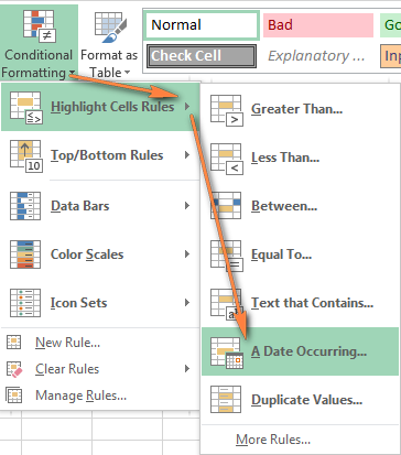
- Select one of the date options from the drop-down list in the left-hand part of the window, ranging from last month to next month.
- Finally, choose one of the pre-defined formats or set up your custom format by choosing different options on the Font, Border and Fill tabs. If the Excel standard palette does not suffice, you can always click the More colors… button.

- Click OK and enjoy the result! : )
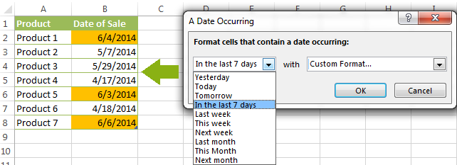
However, this fast and straightforward way has two significant limitations - 1) it works for selected cells only and 2) the conditional format is always applied based on the current date.
Excel conditional formatting formulas for dates
If you want to highlight cells or entire rows based on a date in another cell, or create rules for greater time intervals (i.e. more than a month from the current date), you will have to create your own conditional formatting rule based on a formula. Below you will find a few examples of my favorite Excel conditional formats for dates.
How to highlight weekends in Excel
Regrettably, Microsoft Excel does not have a built-in calendar similar to Outlook's. Well, let's see how you can create your own automated calendar with quite little effort.
When designing your Excel calendar, you can use the =DATE(year,month,date) function to display the days of the week. Simply enter the year and the month's number somewhere in your spreadsheet and reference those cells in the formula. Of course, you could type the numbers directly in the formula, but this is not a very efficient approach because you would have to adjust the formula for each month.
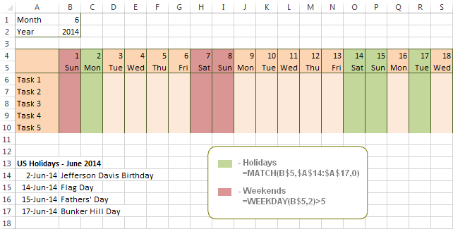
The screenshot below demonstrates the DATE function in action. I used the formula =DATE($B$2,$B$1,B$4) which is copied across row 5.

Tip. If you want to display only the days of the week like you see in the image above, select the cells with the formula (row 5 in our case), right-click and choose Format Cells…> Number > Custom. From the drop-down list under Type, select either dddd or ddd to show full day names or abbreviated names, respectively.
Your Excel calendar is almost done, and you only need to change the color of weekends. Naturally, you are not going to color the cells manually. We'll have Excel format the weekends automatically by creating a conditional formatting rule based on the WEEKDAY formula.
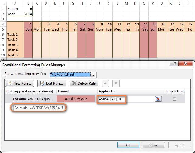
- You start by selecting your Excel calendar where you want to shade the weekends. In our case, it is the range $B$4:$AE$10. Be sure to start the selection with the 1st date column - Colum B in this example.
- On the Home tab, click Conditional Formatting menu > New Rule.
- Create a new conditional formatting rule based on a formula as explained in the above linked guide.
- In the "Format values where this formula is true" box, enter the following WEEKDAY formula that will determine which cells are Saturdays and Sundays:
=WEEKDAY(B$5,2)>5 - Click the Format… button and set up your custom format by switching between the Font, Border and Fill tabs and playing with different formatting options. When done, click the OK button to preview the rule.

Now, let me briefly explain the WEEKDAY(serial_number,[return_type]) formula so that you can quickly adjust it for your own spreadsheets.
- The
serial_numberparameter represents the date you are trying to find. You enter a reference to your first cell with a date, B$5 in our case. - The
[return_type]parameter determines the week type (square brackets imply it is optional). You enter 2 as the return type for a week starting from Monday (1) through Sunday (7). You can find the full list of available return types here. - Finally, you write >5 to highlight only Saturdays (6) and Sundays (7).
The screenshot below demonstrates the result in Excel 2013 - the weekends are highlighted in the reddish colour.
Tips:
- If you have non-standard weekends in your company, e.g. Fridays and Saturdays, then you would need to tweak the formula so that it starts counting from Sunday (1) and highlight days 6 (Friday) and 7 (Saturday) -
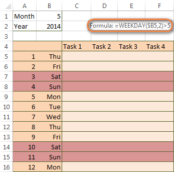
WEEKDAY(B$5,1)>5. - If you are creating a horizontal (landscape) calendar, use a relative column (without $) and absolute row (with $) in a cell reference because you should lock the reference of the row - in the above example it is row 5, so we entered B$5. But if you are designing a calendar in vertical orientation, you should do the opposite, i.e. use an absolute column and relative row, e.g. $B5 as you can see in the screenshot below:
How to highlight holidays in Excel
To improve your Excel calendar further, you can shade public holidays as well. To do that, you will need to list the holidays you want to highlight in the same or some other spreadsheet.
For example, I've added the following holidays in column A ($A$14:$A$17). Of course, not all of them are real public holidays, but they will do for demonstration purposes : )

Again, you open Conditional Formatting > New Rule. In the case of holidays, you are going to use either MATCH or COUNTIF function:
=COUNTIF($A$14:$A$17,B$5)>0=MATCH(B$5,$A$14:$A$17,0)
Note. If you have chosen a different color for holidays, you need to move the public holiday rule to the top of the rules list via Conditional Formatting > Manage Rules…
The following image shows the result in Excel 2013:
Conditionally format a cell when a value is changed to a date
It's not a big problem to conditionally format a cell when a date is added to that cell or any other cell in the same row as long as no other value type is allowed. In this case, you could simply use a formula to highlight non-blanks, as described in Excel conditional formulas for blanks and non-blanks. But what if those cells already have some values, e.g. text, and you want to change the background color when text is changed to a date?
The task may sound a bit intricate, but the solution is very simple.
- First off, you need to determine the format code of your date. Here are just a few examples:
- D1: dd-mmm-yy or d-mmm-yy
- D2: dd-mmm or d-mmm
- D3: mmm-yy
- D4: mm/dd/yy or m/d/yy or m/d/yy h:mm
You can find the complete list of date codes in this article.
- Select a column where you want to change the color of cells or the entire table in case you want to highlight rows.
- And now create a conditional formatting rule using a formula similar to this one:
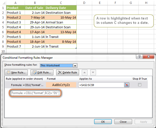
=CELL("format",$A2)="D1". In the formula, A is the column with dates and D1 is the date format.If your table contains dates in 2 or more formats, then use the OR operator, e.g.
=OR(cell("format", $A2)="D1", cell("format",$A2)="D2", cell("format", $A2)="D3")The screenshot below demonstrates the result of such conditional formatting rule for dates.
How to highlight rows based on a certain date in a certain column
Suppose, you have a large Excel spreadsheet that contains two date columns (B and C). You want to highlight every row that has a certain date, say 13-May-14, in column C.
To apply Excel conditional formatting to a certain date, you need to find its numerical value first. As you probably know, Microsoft Excel stores dates as sequential serial numbers, starting from January 1, 1900. So, 1-Jan-1900 is stored as 1, 2-Jan-1900 is stored as 2… and 13-May-14 as 41772.
To find the date's number, right-click the cell, select Format Cells > Number and choose the General format. Write down the number you see and click Cancel because you do not really want to change the date's format.

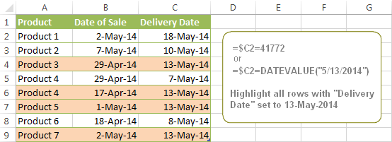
That was actually the major part of the work and now you only need to create a conditional formatting rule for the entire table with this very simple formula: =$C2=41772. The formula implies that your table has headers and row 2 is your first row with data.
An alternative way is to use the DATEVALUE formula that converts the date to the number format is which it is stored, e.g. =$C2=DATEVALUE("5/13/2014")
Whichever formula you use, it will have the same effect:
Conditionally format dates in Excel based on the current date
As you probably know Microsoft Excel provides the TODAY() functions for various calculations based on the current date. Here are just a few examples of how you can use it to conditionally format dates in Excel.
Example 1. Highlight dates equal to, greater than or less than today
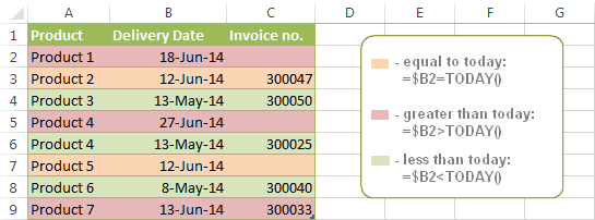
To conditionally format cells or entire rows based on today's date, you use the TODAY function as follows:
Equal to today: =$B2=TODAY()
Greater than today: =$B2>TODAY()
Less than today: =$B2<TODAY()
The screenshot below demonstrates the above rules in action. Please note, at the moment of writing TODAY was 12-Jun-2014.
Example 2. Conditionally format dates in Excel based on several conditions
In a similar fashion, you can use the TODAY function in combination with other Excel functions to handle more complex scenarios. For example, you may want your Excel conditional formatting date formula to color the Invoice column when the Delivery Date is equal to or greater than today BUT you want the formatting to disappear when you enter the invoice number.
For this task, you would need an additional column with the following formula (where E is your Delivery column and F the Invoice column):
=IF(E2>=TODAY(),IF(F2="", 1, 0), 0)
If the delivery date is greater than or equal to the current date and there is no number in the Invoice column, the formula returns 1, otherwise it's 0.
After that you create a simple conditional formatting rule for the Invoice column with the formula =$G2=1 where G is your additional column. Of course, you will be able to hide this column later.

Example 3. Highlight upcoming dates and delays
Suppose you have a project schedule in Excel that lists tasks, their start dates and durations. What you want is to have the end date for each task calculated automatically. An additional challenge is that the formula should also consider the weekends. For example, if the starting date is 13-Jun-2014 and the number of days of work (Duration) is 2, the ending date should come as 17-Jun-2014, because 14-Jun and 15-Jun are Saturday and Sunday.
To do this, we will use the WORKDAY.INTL(start_date,days,[weekend],[holidays]) function, more precisely =WORKDAY.INTL(B2,C2,1).
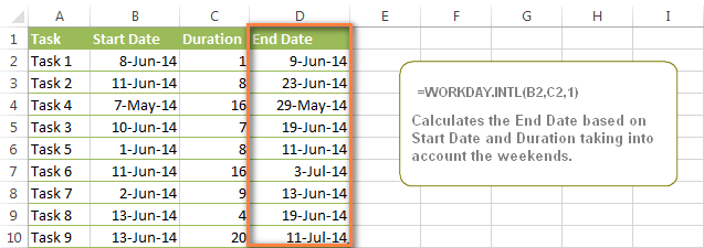
In the formula, we enter 1 as the 3rd parameter since it indicates Saturday and Sunday as holidays. You can use another value if your weekends are different, say, Fri and Sat. The full list of the weekend values is available here. Optionally, you can also use the 4th parameter [holidays], which is a set of dates (range of cells) that should be excluded from the working day calendar.
And finally, you may want to highlight rows depending on how far away the deadline is. For example, the conditional formatting rules based on the following 2 formulas highlight upcoming and recent end dates, respectively:
=AND($D2-TODAY()>=0,$D2-TODAY()<=7)- highlight all rows where the End Date (column D) is within the next 7 days. This formula is really handy when it comes to tracking upcoming expiration dates or payments.=AND(TODAY()-$D2>=0,TODAY()-$D2<=7)- highlight all rows where the End Date (column D) is within the last 7 days. You can use this formula to track the latest overdue payments and other delays.
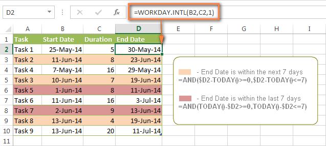
Here are a few more formula examples that can be applied to the table above:
=$D2<TODAY() - highlights all passed dates (i.e. dates less than the current date). Can be used to format expired subscriptions, overdue payments etc.
=$D2>TODAY() - highlights all future dates (i.e. dates greater than the current date). You can use it to highlight upcoming events.
Of course, there can be infinite variations of the above formulas, depending on your particular task. For instance:
=$D2-TODAY()>=6 - highlights dates that occur in 6 or more days.
=$D2=TODAY()-14 - highlights dates occurring exactly 2 weeks ago.
How to highlight dates within a date range
If you have a long list of dates in your worksheet, you may also want to highlight the cells or rows that fall within a certain date range, i.e. highlight all dates that are between two given dates.
You can fulfil this task using the TODAY() function again. You will just have to construct a little bit more elaborate formulas as demonstrated in the examples below.
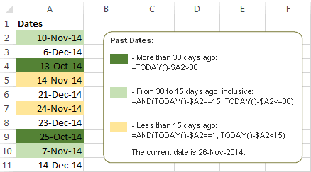
Formulas to highlight past dates
- More than 30 days ago:
=TODAY()-$A2>30 - From 30 to 15 days ago, inclusive:
=AND(TODAY()-$A2>=15, TODAY()-$A2<=30) - Less than 15 days ago:
=AND(TODAY()-$A2>=1, TODAY()-$A2<15)
The current date and any future dates are not colored.
Formulas to highlight future dates
- Will occur in more than 30 days from now:
=$A2-TODAY()>30 - In 30 to 15 days, inclusive:
=AND($A2-TODAY()>=15, $A2-TODAY()<=30) - In less than 15 days:
=AND($A2-TODAY()>=1, $A2-TODAY()<15)
The current date and any past dates are not colored.

How to shade gaps and time intervals
In this last example, we are going to utilize yet another Excel date function - DATEDIF(start_date, end_date, interval). This function calculates the difference between two dates based on the specified interval. It differs from all other functions we've discussed in this tutorial in the way that it lets you ignore months or years and calculate the difference only between days or months, whichever you choose.
Don't see how this could work for you? Think about it in another way… Suppose you have a list of birthdays of your family members and friends. Would you like to know how many days there are until their next birthday? Moreover, how many days exactly are left until your wedding anniversary and other events you wouldn't want to miss? Easily!
The formula you need is this (where A is your Date column):
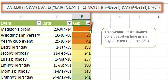
=DATEDIF(TODAY(), DATE((YEAR(TODAY())+1), MONTH($A2), DAY($A2)), "yd")
The "yd" interval type at the end of the formula is used to ignore years and calculate the difference between the days only. For the full list of available interval types, look here.
Tip. If you happen to forget or misplace that complex formula, you can use this simple one instead: =365-DATEDIF($A2,TODAY(),"yd"). It produces exactly the same results, just remember to replace 365 with 366 in leap years : )
And now let's create an Excel conditional formatting rule to shade different gaps in different colors. In this case, it makes more sense to utilize Excel Color Scales rather than create a separate rule for each period.
The screenshot below demonstrates the result in Excel - a gradient 3-color scale with tints from green to red through yellow.
"Days Until Next Birthday" Excel Web App
We have created this Excel Web App to show you the above formula in action. Just enter your events in 1st column and change the corresponding dates in the 2nd column to experiment with the result.
If you are curious to know how to create such interactive Excel spreadsheets, check out this article on how to make web-based Excel spreadsheets.
Hopefully, at least one of the Excel conditional formats for dates discussed in this article has proven useful to you. If you are looking for a solution to some different task, you are most welcome to post a comment. Thank you for reading!
 by
by
1201 comments
Hello,
I am trying to make a formula where I want the cell to be highlighted when it says "In Progress" and the date is past 14 days.
Column C is the date posted, and Column E is the status column (Ready, In Progress, ect.)
This is the formula I thought would work, but am getting an error message:
=AND(TODAY()-C3>=14, E3 = “In Progress”)
The error I'm getting says "you may not use reference operators (such as unions, intersections, and ranges), array constants, or the LAMBDA function for conditional formatting criteria."
Hi!
I assume you used the wrong quotes for the text string.
Use the formula:
=AND(TODAY()-C3>=14, E3 = "In Progress")
I have a spreadsheet that I need help with.
I need to highlight the cell if a date entered is within the current quarter.
Qtr1 Oct-Dec
Qtr2 Jan-Mar
Qtr3 Apr-Jun
Qtr4 Jul-Sep
If not, then highlighted red. If so, then highlighted green.
Hi!
You can determine the quarter number by date using the MONTH function and rounding.
=ROUNDUP(MONTH(A1)/3,0)
You can define a partial match of the quarter number with the text by using a formula like this
=ISNUMBER(SEARCH(ROUNDUP(MONTH(A1)/3,0),B1))
For more information, please read: How to find substring in Excel
I'd like to format cells to highlight based on a date range not related to today's current date (e.g., highlight all cells with dates from June 2022-December 2022 with one color, highlight January 2023-June 2023 with a different color, etc.). The tricky part is the dates I want referenced are on sheet 2 and the cells I want formatted are on sheet 1. Is this something that is possible?
Hello!
To correctly use references to cells from another worksheet in a formula, see these guidelines - Excel reference to another sheet or workbook (external reference).
I have a spread sheet with notes being taken daily with dates input using CTRL ;
these dates are mixed in with notes Example. 06/03/2023 important information here
I was wondering if there is a way at all to highlight or change the text color of the date only automatically without changing the text of the entire cell or color of cell?
Hi!
Unfortunately, you can only change a part of the cell formatting manually or with VBA.
Hello, I am looking for help on a conditional format:
- I have a column (E8) for a deadline and a column (D8) for progress. Progress column is formatted as a percentage and conditionally formatted as a data bar (so will show a progress bar based on percentage entered). I am trying to highlight cell in the deadline column (E8) when deadline is overdue AND Progress column(D8) is less than 100%. I also want to ignore all blanks but I have a format for now that place ignoring blanks higher up on the hierarchy of formatting. Any suggesting for a formula would be great appreciated as I have tried numerous with no success,
Hi!
I’m sorry but your description doesn’t give me a complete understanding of your task. Correct me if I’m wrong, but I believe the conditional formatting formula below will help:
=AND(D8<1,E8<today())
You can also find useful information in this article: Apply multiple conditional formatting rules to same cells.
IF I HAVECHANGE DATE ,EFFICIENCCY CALCULATE WITH CHANGES DATE WHAT CONDITION USED
Good Day,
I hope you can help.
I have a client Data base. I have a coloumn (Last Groomed) = (G) and (Next Groom) = (H). Due to the nature of my business the client will tell me when the next groom will be or if it is a monthly standing booking.
So the formula i have in H is as such (=G3+30) which will give me 30 days from today.
So what i need is a rule / format / Formula, that highlights cells 10 days before (Today)=(A1) (in Orange) and 10 days after (Today)=(A1) automatically when i open the workbook.
Thank you your assistance is appreciated
Hi!
Pay attention to the following paragraph of the article above – Conditionally format dates based on the current date.
For example,
=$A1-TODAY()>=10 - highlights dates that occur in 10 or more days.
Hi
may I have some help please.
Job Number Job Description Booking Date Target Date Completed Date Additional Notes
1 test 14/02/2023 25/01/2024 14/02/2023 Done
How do I make the entire row green once a 'completed date' has been inputted?
there is a conditional format for target date which works perfectly and I don't want to disturb that.
Kind regards,
Abdul
Hello!
Create another conditional formatting rule using this instruction: How to change the row color based on a cell's value. I hope it’ll be helpful.
I have a list of dates and I want to color the cells which contain the dates, conditionally every time the year changes. So, all of 2023 would be one color and all of 2022 would be a different color, and on and on. But, these cells are a complete date, for example, 02/10/2023, so I need to learn how to just extract the year from these cells and conditionally format based on only the year. Thanks for your help.
Hi!
Use the recommendations from the article above. To determine the year, use the YEAR function. Try a conditional formatting formula like this:
YEAR(A1)=2022
I have dates from the early 1900s through today, hundreds of rows, each year having a different quantity of rows. Is there a way for conditional formatting to automatically have Excel assign a different color based on which year it is? It would take forever to write an individual formula for 100+ years. Or if there is a way to highlight all 2023 rows in one shade of grey and then all of 2022 in another shade and then 2021 back to the shade of grey of the 2023 years? I'm just trying to visually see when the year changes and which rows are included in that particular year.
Hello!
You need to create a separate conditional formatting rule for each color. To make this rule work for different years, use the logical OR function.
=OR(YEAR(A1)=2023,YEAR(A1)=2021,YEAR(A1)=2019)
or
=SUM(--(YEAR(A1)={2023,2021,2019}))
Rule for all odd years -
=MOD(YEAR(A1),2)=1
Rule for all even years -
=MOD(YEAR(A1),2)=0
I hope it’ll be helpful.
I am setting up a spreadsheet that will be keeping track of animal licensing information:
id#
owner name
pet name
expiration date of vaccine
expiration date of license
ect...
I am looking to make certain cells change to colors depending on the dates of the license expiration and or if I change the status of the owner. currently it is sep up as such:
A- last name
B-first name
C-license status (drop down list for the following options - expired, current, in progress, township sending notice and attending clinic)
D-date license expires
E- phone
F- house #
G-street address
H- township located
I-last vaccination date
ect...
I need to set up a system where:
anything before 10/31/22 (or 44865) turns red
anything between 11/1/22() and 1/31/23 (44957) turn yellow
and anything up to now turns green
I also want to be able to change the status colomn and have it effect the color. so if a license is expired but the owner is trying to go to a clinic I can choose attending clinic in colomn c and it will change it to an overriding color to indicate that status. Is this possible?
Hi!
Have you tried the ways described in this blog post? Create a rule for each color according to the recommendations in the article above.
I have tried several of the methods but I cant figure out how to make it conditional, ie-when cell turned on then the color is turned on but when off the color turns off.
Hi!
What does "cell turned on" mean? What cell conditions are you checking for? What are those conditions? I can't guess.
So with a drop down box there are two options-ON, OFF. when I select the option for on in a cell I want a color to appear in a row of cells designated. for example if I want to have a cell that is for EXPIRED animal licenses. I have a box colored red that states expired and a drop down box in the cell below it with ON and OFF. when the second cell states on I want all the cells in another box that say EXPIRED to turn red. When the cell is turned OFF I want the cells to go back to no color.
Hi!
If I understand your task correctly, try the following conditional formatting formula:
=AND(D2="Expired",$F$1="on")
MAYBE I AM NOT UNDERSTANDING BECAUSE I CANNOT GET IT TO FORMAT CORRECTLY. COULD I INSTEAD HAVE FOR EXAMPLE D CELLS DECIDE ON THE ACTION OF THE C CELLS? SO IF A DATE IS EXPIRED IN THE D CELL THEN THE C CELL WILL AUTOMATICALLY SAY EXPIRED AND TURN RED? WITH THE OPTION TO CHANGE THE COLOR IF PROGRESS IS PENDING? THIS MIGHT BE A BETTER IDEA. DOES THAT MAKE SENSE?
Hi!
You can change the value in cell C2 depending on the date in D2 with the formula =IF(D2<TODAY(), "off", "expired") You can change the color of C2 with the conditional formatting formula =D2<TODAY()
But if cell C2 contains a drop-down list, this cannot work.
ok so if my cell for c is c6 and I am doing
cell value is equal to ="EXPIRED"
and my D cell value is between =41305 and =44865
then would my new c value be ="EXPIRED" =IF(D2=
im not sure how to add the varience in the newly made format. it would have to show the cell value is equal to = EXPIRED but also add only if its between the numbers 41305 and 44865
For a multi-condition formula, use these guidelines: IF AND in Excel: nested formula, multiple statements.
=IF(AND(D2>41305,D2<44865),"expired","")
So if I am understanding correctly than my formulas would be the following:
=IF(AND(D2:D125>41305,D2:D12544957,D2:D12544865,D2:D125<44957),"township sending notice")
noting that these values are dates but were turned into numeric for easier formula use but show as dates on the excel sheet
Is there a way to dynamically change cells according to time instead? I am working with a daily schedule and I would like to see what is happening at what hour when I look at it.
Hi!
I'm really sorry, looks like this is not possible with the standard Excel options.
So I have a worksheet that shows production data on a calendar. The dates are pulled from a website so they will auto rotate which cell shows which dates. I use this sheet to see when I can schedule new orders to ship. This also depends on what shipping routes are available. I have created a new tab with all my routes and and their schedules.
I have added a drop down on my main page to select the route. Now I want to highlight cells in the schedule based on which route is selected.
My excel terminology is limited so I will attempt to describe the formula I am looking for;
Rule 1) If this route is selected then highlight all Tuesday/Fridays
Rule 2) if this route is selected highlight all Monday/Wednesdays
-so on and so forth for other routes and their respective days.
I cannot find the formula excel needs to make this happen. Am I overthinking this and there is a simple solution/equation? or is this something excel cannot do?
Hello!
Use the WEEKDAY formula to determine the day of the week. For example, conditional formatting formula:
=OR(WEEKDAY(A1,2)=2,WEEKDAY(A1,2)=5)
Thanks, yes I was able to get the correct days highlighted using this equation:
=OR(WEEKDAY($B2,2)=3, WEEKDAY($B2)=2)
The tricky part for me is having this contingent on a cell showing different route options. For example:
If i select "ALL01" then Tuesdays and Thursdays will highlight
If i select "CHI01" then Tuesdays and Fridays need to highlight
The selections is being made in a drop down i created.
The "ALL01" & "CHI01" are routes we use.
Hi!
Add another AND condition:
=AND($M$1="ALL01",OR(WEEKDAY($B2,2)=4, WEEKDAY($B2,2)=2))
Hazaaa!!!
That worked - thank you so very much!!
Hello!
I am using the conditional formatting steps detailed above for past dates, future dates, and todays dates. However the formulas do not seem to be working. What do I do?
Hi!
I can't know what you are doing in your workbook. Note that the dates are written as dates and not as text. Follow the instructions in the article above carefully.
Help! I really hope you can respond to this and help me!
I need a formula(s) to apply conditional formatting based on various dates in a column both on the same tab and from a previous tab in the same workbook. Column A is "Date Received" (where the date will vary by when something was received). Column B would be Date Created.
The basics of the formula I need would be if Column A date is greater than 1 week (or 7 days, whichever is easier), format the cell yellow, if greater than 2 weeks (14 days), format the cell red.
Specific Example: If a date isn't entered in Column B within one week (or 7 days, which ever is easier), the cell in Column A will turn yellow, if no date is entered in Column B within 2 weeks (or 14 days) the cell in Column A will turn Red. If a date is entered in Column B the cell in Column B with the date can turn green.
The ideal formatting would be to add icon sets with with the stop lights instead of highlighting the cell with a color. I believe there is an option to enter a custom formula to apply it with the icon sets, correct? If so, I will do that using the formula above. If not, it's not a deal-breaker.
One other thing, how do I reference a column from another tab so it will add and show two weeks after the date in a column of the other tab. Example - Column A "Quote for Approval" in Tab 1 has a date entered for when the quote was submitted. We need Column B in Tab 2 to add 2 weeks (14 days) and put that in Column A from Tab 1. The conditional formatting for that date in Tab 2 would be based on the original date in Tab 1 but would be the same concept of >7 days, >14 days.
I really hope this makes sense. Please let me know if you have questions and thank you very much for having the forum!!!
Hello!
Date-based conditional formatting is detailed in the article above. You may also be interested in this article: Excel Icon Sets conditional formatting: inbuilt and custom.
Hi Alexander Trifuntov (Ablebits Team)
I'm trying to make a scheduling template for 18 employees. I can't figure out how I can auto-highlight the scheduled time (interval of 9 hours) when I put the shedule in a different cell, then also apply a different color when I type in a break time in a different cell as well.
F4 - schedule (9am-6pm)
F4 - 1st break (11 am)
G4 - Lunch start (1pm)
H4 - Lunch End (2pm)
I4 - 2nd break
Trying to apply the formatting to K4-BF18, every cell from J4 is considered a 15 min interval.
Also, I would like to change the color of each cell within the time range when agent's status in J4 is absent or late. I hope you can help me. Thank you so much in advance!
Hi!
Sorry, I do not fully understand the task. What formatting do you want to apply in K4? Why are there two values in F4? What does it mean "agent's status in J4 is absent or late"?
When we entering date 1/1/30 in excel its returning 1/01/1930 or 1/1/40 its returning 1/01/1940.I am expecting 01/01/2030 or 01/01/2040 in this case.Is it possible to fix this using conditional formating.I need to fix this in excel only.Can you please let me know best possible way.
AlexChanged system date settings.Still it’s not working.
Hello!
Set the cell to the date format you want. For example - dd/mm/yyyy. Use these guidelines: How to change Excel date format and create custom formatting.
Thank you Alex. My cell has value 31-DEC-30 ,Converted cell to date format DD-MON-YYYY .Its converting to 31-DEC-1930. Getting year wrong in Excel 2016.I have column formula =IF(ISBLANK(X89),"",DATEVALUE(X89)).
Issue:
30 through 99 is interpreted as the years 1930 through 1999. For example, if you type the date 5/28/98, Excel assumes the date is May 28, 1998.
Hi!
Your problem is described here: Fixing dates with two-digit years.
Or create a date with the DATE function:
=DATE("20"&RIGHT(A1,2),MONTH("1"&MID(A1,4,3)),LEFT(A1,2))
Hello. I have three columns of dates (all on the same row). I need column C to highlight green if the date is before both dates in columns A and B, highlight yellow if it’s before only one date (A or B) and past the other date (A or B), and highlight red if it’s past both dates A and B.
Hello!
Create 3 conditional formatting rules using these formulas:
=AND(B1>C1,A1>C1)
=((C1>B1)+(C1>A1))=1
=AND(B1<C1,A1<C1)
I hope my advice will help you solve your task.
I need to figure out how to have a date change color after the date has reached 6 months and a different color for when its been 1 year. This is dealing with date of employment and the 6 month and year bench marks are for raises.
The date conditional formatting only goes back a month.
Would also be amazing if when the color changes that it sparks an email to the hiring manager.
Hi!
Please re-check the article above since it covers your case. Sending an email automatically is possible with a VBA macro.
I need to conditional format cells so that they are automatically coloured in when the date changes in the first column.
I have used the eomonth formula in a col before the calendar date rows start. If I change the date on cell b10 then the eomonth formula gets updated in cell e10.
I need the the next section which the dates Jan to Dec per year sections to highlight cell accordingly to the date in cell b10.
Hi!
Based on your description, it is hard to completely understand your task. To determine the month, try the MONTH function.
Hi, I'm trying to set up conditional format for a specific time range between 0-10 hours , Kindly assist with best approach.
Thanks in anticipation
Thank you for taking the time to put this together. It is helpful for highlighting holidays. However, if a holiday falls on a Saturday or Sunday my agency observes the holiday on the Friday prior, or Monday after. Is there a way to have excel highlight the Friday prior to a Saturday holiday, or the Monday after a Sunday holiday?
Hello --
Not sure if I'm following the right thread. But I'm in Google Sheet and I have the same exact problem.
I wanna highlight cells that match another set of cells.
For example : cell E4:O4 contains time - and below them are E8:M399 with time as well. And I want to highlight the time in cell E8:M399 to match E4:O4..
I'm using =match(E8,indirect("SCHEDULE & COVERAGE!E4:O4"),0) applied to range E8:M399
It actually works to all cells except if the time from E8 starts with 12am or 0:00
It works if the time 12am or 0:00 is in the middle for example J8..
Hi,
How do I highlight a course date that is due to be renewed. Let say, I attended a course on the 1/11/2022. And the course has to be renewed after 3 years which is 1/11/2025. What can I do to highlight the course date if the actual date is 3 months before the renewal date i.e > 1/8/2025? Thank you
Hi!
Please reread the article above since it covers your case.
Hi,
I have a Gantt chart issue and I’m wondering if you could help?
I have a Task Start Date Column (C), End Date Column (D), and Progress % (E). If the Task Progress (Cell E1) is still 0% after the task start date (Cell C1), is it possible to highlight the start date (Cell C1)?
I hope that makes sense.
Thanks
Hi,
How do I highlight the cells that are within the 9 hour shift per 1 hr interval. I already have the count which decreases when an employee ended the shift.
Example: there are 5 employees logged in by 3pm. And within 3pm, it consist of the shift from 6am to 2pm. I would like to check if it is possible to highlight those 5 employees.
Hi!
If I understand your task correctly, try the following conditional formatting formula with logical function OR:
=OR(A1>=TIME(15,0,0),A1<=TIME(5,0,0))
Hello --
Not sure if I'm following the right thread. But I'm in Google Sheet and I have the same exact problem.
I wanna highlight cells that match another set of cells.
For example : cell E4:O4 contains time - and below them are E8:M399 with time as well. And I want to highlight the time in cell E8:M399 to match E4:O4..
I'm using =match(E8,indirect("SCHEDULE & COVERAGE!E4:O4"),0) applied to range E8:M399
It actually works to all cells except if the time from E8 starts with 12am or 0:00
It works if the time 12am or 0:00 is in the middle for example J8..
I am needing to compare due dates and completion dates. I am specifically trying to have it automatically generate a green for on time and red for overdue. This is so that I may be able to easily notice trends within specific departments. I am having difficulty with dates that are the same as the due dates and with not having to format each entry. I would appreciate any and all assistance. Thank you.
Hi!
Have you tried the ways described in this blog post? Please describe your task in detail if they don’t work for you.
I need a condition like previous month of 9th to current date is this possible in excel and every time previous month will be changed like this is october then the previous moth is september if the month is december then need to extract data from november 9th to current date
Hi!
To determine the 9th of the previous month, try the formula
=DATE(YEAR(EOMONTH(TODAY(),-1)), MONTH(EOMONTH(TODAY(),-1)), 9)
Here is the article that may be helpful to you: How to add and subtract dates in Excel.
Hi - I may be in the wrong place for this question, so apologise if I am.
I am pasting a number of dates from a genealogy programme into an Excel worksheet. Some of the dates are day/month/year, some are month/year and some are just year. How do I format the column so they appear as they should do?
If I format for day month year, then the "year only" dates are miss-interpreted, eg 1924 becomes 07/04/1905
If I format for number, 01/07/1916 becomes 6027.
Is there a conditional format solution to this?
Thanks
Jeremy
Hello!
1924 is a number, not a date. To get the date, you can use these recommendations: How to convert number to date in Excel. To convert a year number to a date, use the DATE function. For example,
=DATE(A1,1,1)
If you have a lot of different values that need to be converted to date, try Text to Date tool. It is available as a part of our Ultimate Suite for Excel that you can install in a trial mode and check how it works for free.
Alexander thanks - I understand what you are saying but I can't find a simple way of formatting the column to display a consistent date when the input data is in 3 different formats (as described). I'll have a play and eg see if I can display all dates as simply a year eg 1950. I believe I may be able to do this by format/number/custom/ then type in yyyy?
Jeremy
Hi!
Please provide me with an 5-6 examples of the source data and the expected result.
Hi Alexander,
In my column G I want all contract dates, expiring in less than 6 months highlighted in conditional formatting. I already found some codes but I'm receiving a "There's a problem with this formula." error. Maybe is it because I'm working on a macbook?
Can you please help me? Thanks
Hi!
Which formula is the problem? Write it down.
Hi!
How can I format the cells containing hour info to indicate it started or ended according to the current time.
Example;
NOW() : 10:30
START END
event 1 11.11.2022 08:40 09:30 start and end should be coloured
event 2 11.11.2022 08:40 11:30 start should be coloured
event 3 11.11.2022 10:40 12:30
event 4 11.11.2022 14:40 16:30
Hi!
You can find the examples and detailed instructions in article above.
The NOW() function returns the date and time. To use time only, apply the formula
NOW()-INT(NOW())
Use conditional formatting rule:
(A1-INT(A1))<(NOW()-INT(NOW()))
I hope this will help.
I have used conditional formatting on a spreadsheet. In it I have it set to figure the number of days since a unit has been cleaned and color code it to let me know how close it is to needing to be re-cleaned. My problem is that in the units that are rented, I did not populate the date of cleaning so it has no date to judge by and has put in a date of 6/28/1900. I am sure this is set up in the system but I want to find out how to set the cell up so when the date is left off it does not calculate anything and leaves the date blank. The formula I have used is: =(D+180) D is the ce3ll where I input where each unit was last cleaned. I want the cell to populate only if there is something in the D column.
Hi!
If I understand your task correctly, you can use IF function to check value of cell D1.
=IF(D1<>"",D1+180,"")
Hope this is what you need.
How can i entire row fill with color by conditional format when put in there random date in excel?
Plz give some clue & more easier if you send some snapshot..?
Hi!
The following tutorial should help: How to change the row color based on a cell's value in Excel.
If we have a start date with timing and end date with timing how to highlight colors very close to end time.
Hi!
Have you tried the ways described in this blog post? Please re-check the article above since it covers your task.
Hello sir,
I'm preparing sheet name issued material list and i want to apply condition formatting on this sheet
ex. i issued one shoes or helmet on current date n the reissued time is 6month
i want to apply condition on current date
the color will be change when it expire . can u plz help me
Hi Alex,
Great post!
I would like to alternate colors of date range based on fiscal year from June to July (following year).
Many thanks in advance.
Hi all,
How do I change the colour of a value based on how the number of that value in the column?
Eg if date 01/01/22 appears in a column 5 times it will turn orange. But when that date appears 8 times it will turn red.
Thanks
Hi!
Create a separate conditional formatting formula for each color. To count the number of values in a column, use the COUNTIF function -
=COUNTIF($A$1:$A$100,A1)=5
Hope this is what you need.
Hello,
I have created a spreadsheet and applied conditional formatting to my date column to highlight all future dates using the example above '=$B2>Today()'. For some reason it isn't picking up all of them.
In one instance, when I sort by date it will highlight all future dates with the exception of the last row. That row will highlight if I add a future date to the row directly under it but the new future date will not be highlighted.
If I resort by job number (different column) some of the previously highlighted dates are now not highlighted.
I've confirmed the date column is all formatted correctly. I'm using Office 365 if you think that might be causing the problem.
Thank you in advance for any help you can provide.
Hello!
The row number in the conditional formatting formula must match the number of the first row of the conditional formatting range. For example, for the range B1:B100 or B:B, you need to use the formula
=$B1 > Today()
Your formula "=$B2 > Today()" will work for a range, for example, B2:B100.
I hope I answered your question. If something is still unclear, please feel free to ask.
We have dates in column D. We would like to add a condition when it is 1 week past the date it changes colour, then again when 2 weeks past date to a different colour and again when its past 3 weeks. What formula would use per week?
Thanks,
Kasey
Hi!
Please re-check the article above since it covers your task. Pay attention to the following paragraph: Conditionally format dates based on the current date.
Hi,
So I have a task list, and I want to use conditional formatting for two things. Number one, I want to highlight a cell that has been left blank in a range past a due date to complete the task. I have that due date represented in a cell in the same sheet, in case I need to make reference to that date in the conditional formatting formula. Additionally, I want to also highlight cells that reflect a date past that same due date, within the same range.
I am having the hardest time, because all of the formulas I find use a moving date, usually in relation to today, or weekends, or holidays. I believe what I need should be much simpler than those. Help!
Ok ok... I solved the the second part of my question with a pre-made, greater than formula. Still... the first formula I still don't know how to do it.
As a reminder, I need the cells in a column to light up if the date on a cell that I will be updating every month has passed, and the cells in that column are blank, indicating the task has either not been completed, or the employee has not recorded their task. Please help.
Hi!
The logical AND function can combine two conditions. For example,
=AND($B2
Hi!
Have you tried the ways described in this blog post? Pay attention to the following paragraph of the article above - Conditionally format dates in Excel based on the current date. If they don’t work for you, then please describe your task in detail, I’ll try to suggest a solution.
i have put this formula in my excel conditional formation but it show me date of one day before Sunday. =WEEKDAY($B3,2)>6
please can you help me out.
Hi!
I don't really understand what you want to do. Your formula shows TRUE if the date is Sunday. I recommend paying attention to the examples of the WEEKDAY function. Or explain the problem in more detail.
Hi All
I really need your help.
I have an inventory in and out log. It logs date an asset was issued and date it was returned. I have everything in a drop down menu and i need the following. these assets are loaned out on a daily basis and returned on a daily basis. (Or supposed to be) there are other assets issued on a semi permanent basis
My drop down items on another sheet are (data validation):
Issued (Conditional Formatting Turns the Cell Yellow if issued is selected)
Returned (Conditional Formatting turns the cell Green if returned is selected)
Semi-Permanent (Conditional Formatting turns the cell orange if semi-permanent is selected)
Lost (turns red when selected)
Stolen (turns purple when selected)
If the cell with the date issued is today, the cell containing the selected status "Issued" turns yellow. Issued is a drop down item on another sheet.
If the cell with the date issued is older than today and the status of the asset still says issued I want the cell to change from yellow fill saying Issued, to Red fill and say "OVERDUE" in bold white. OVERDUE is not a drop down item on another sheet.
Essentially every night at midnight i want the status of the assent issued.
Perhaps i should add OVERDUE to the drop down items but im really not sure
Hello!
The value in a cell with a drop-down list cannot be changed automatically. To change the value in a cell to “OVERDUE” according to the conditions, use the IF AND combination. You can change the color of this cell with conditional formatting.
Hi,
I have a table which contains two columns with dates. I want to highlight in one of the columns the dates that are greater with 3 or more days than the dates în the other column. How can i do this?
Thank you.
Hello!
If you want to highlight dates in column B, then apply a conditional formatting rule to it with formula:
=B1-A1>3
This should solve your task.
Hello,
I am trying to create an expense reimbursement sheet for my office.
I have a date column (to indicate when the expense was incurred), that people will manually fill.
I would want a "Period" section that automatically fills out depending on those dates.
i.e. An employee incurred expenses 03/01/2022 and 04/05/22. How can the period section automatically change to "03/01/2022-04/05/2022."?
Thank you so much!
Hello!
You can convert a date to text with the TEXT function. Then concatenate these two dates into a text string using the CONCATENATE function or the & operator.
=TEXT(A1,"dd/mm/yyyy")&" - "&TEXT(A2,"dd/mm/yyyy")
I hope it’ll be helpful.
Thank you!
So I have done that, the issue is that the second "A2" will be changing depending on the number of items, that they will enter, so it sometimes will be A3 or A4, or A5, etc. I have also tried doing a Min Max and concatenate, but I feel I'm missing a part on that second part.
Hello!
If you have several dates in a column, then I recommend paying attention to this instruction: Look up a value in the last non-blank cell in a column.
I hope I answered your question. If something is still unclear, please feel free to ask.
Hello there!
I am trying to highlight cells using different colors, based on how far away they are, both upcoming and having passed.
Scenario: I have a deadline for an agreement listed in my spreadsheet. The day is coming up and I would want it to turn yellow when it is 2 weeks away and red when it is one week away or less.
Scenario 2: I have a date that has passed and I would want it to turn say orange when that date is 3 weeks ago, then red when it is over a month ago.
I have found things that seem like they should work, using formulas like =TODAY()-C4>30 but I can't seem to make them work.
Please help. Thank you.
Hello!
Have you tried the ways described in this blog post? Unfortunately, I can't create conditional formatting in your table. If you want to highlight other cells based on the cell with the date, then I recommend that you study this instruction.
(duplicate and corrected)
I stopped reading at September 2021. Appreciate the time you take to answer the inquiries. Thank you. I couldn't find how to answer my question in some of the replies and am not familiar with Excel or formula use except little by little over time. My question is:
I have been using the COUNTIF to find specific text within a cell. I am *now trying to do the same with the date, specifically the last 30 days. So within a text, there will be a date followed by a varied comment. I am trying to yellow fill and red annotate that comment for the last 30 days.
If you can assist, please advise.
-THANK YOU
Hello!
To find specific text in a cell, it's best to use the SEARCH and FIND functions. Your explanations are not very clear. But to set the background of a date cell with a specific color, use this article's recommendations. However, it is not possible to change the color of only part of a cell.
If date and comment are written in the same cell, then you need to extract the date from the text: Regex to extract date from string.
Describe your problem in more detail and maybe I can help.
Hi, i need help to create a conditional formatting rules that automatically highlights that date before 3 months , like if its 14/01/23 it highlights it when 14/11/22 . Can you help me , i did read the tutorial but i dont understand , can you give the simple sample rules.
Hi!
Pay attention to the following paragraph of the article above - How to highlight dates within a date range.
Formula to highlight future dates more than 90 days from now: =$A1-TODAY()>90
You can also add 3 months to the current date and compare it to the date in the cell:
=DATE(YEAR(TODAY()),MONTH(TODAY())+3,DAY(TODAY()))>A1
The following tutorial should help: Subtract dates in Excel; add days, weeks, months or years to date.
Hello,
Used the formula listed in this article:
=AND(TODAY()-$D2>=0,TODAY()-$D2<=7) - highlight all rows where the End Date (column D) is within the last 7 days. You can use this formula to track the latest overdue payments and other delays. (I changed it to 120 days to see upcoming due dates within the next 4 months)
But it only highlights the cell, not the row? How do I change it to highlight the row?
Thank you!
Hello!
When creating a conditional formatting rule, select the entire range of cells that you want to highlight with color. For example, A2:N50
Then create a rule with your formula.
Try to use the recommendations described in this article: How to change a row color based on a number in a single cell.
Hello,
I hope this is easy and straightforward...I have a date column and I'd like to create another date column, but I'd like it to show the date that is 4 months ahead of the first date column. This would be part 1 of my question.
Part 2 would then be, how can I get the row to change colour, once the date in this new column is going to occur in the next four months?
Explanation: What I am trying to do is have rows be highlighted when a specific item is coming due within the next four months so that it will be visually flagged.
Thank you for your time!
Hello!
Read the answer to the first question in this article - Add months to date in Excel.
=DATE(YEAR(A2), MONTH(A2) + 4, DAY(A2))
If the formula is written in column B, then you can use row conditional formatting:
=DATE(YEAR(TODAY()), MONTH(YEAR(TODAY()) + 4, DAY(YEAR(TODAY()))>$B2
I recommend reading this guide: How to change the row color based on a cell's value.
I hope my advice will help you solve your task.
Thank you! :-)
hi,
Im not sure why the following conditional formating formula doesnt work. Cell tresults in the table are references and formulas. No errors are reported when saving but nothing gets highlighted. I was expecting the 5th row (04/05/22 08:47 23/05/22 15:57) to get highlighted
=AND($G5>NOW(),$H5<NOW())
Colum G Column H
Start Date Date Calc
04/05/22 08:47 04/05/22 08:47
04/05/22 08:47 04/05/22 08:47
04/05/22 08:47 04/05/22 08:47
04/05/22 08:47 04/05/22 08:47
04/05/22 08:47 23/05/22 15:57
23/05/22 15:57 02/08/22 23:48
02/08/22 23:48 13/10/22 07:38
13/10/22 07:38 23/12/22 15:28
23/12/22 15:28 04/03/23 23:19
04/03/23 23:19 15/05/23 07:09
15/05/23 07:09 10/12/40 16:46
ahhhh pls ignore the comment/question. just had the wrong way arround.
Hi!
The second condition in your formula returns FALSE. Therefore, the AND formula also returns FALSE.
Hi There! I've built two sheets in the same workbook: first, a list of teammates, their start date of travel, and the end date of travel. Second, I built a sheet with a calendar similar to yours above with "tasks," but instead it has team members in the first column. I would like the calendar to highlight the dates each team member is traveling referenced from the first sheet. Do you know how I'd do this? Thank you!
Hello!
I don't think that your problem can be solved with conditional formatting. Try using a Gantt chart. I recommend reading this guide: How to make a Gantt chart in Excel. I hope my advice will help you solve your task.