 by
by If you are a regular visitor of this blog, you've probably noticed a few articles covering different aspects of Excel conditional formatting. And now we will leverage this knowledge and create spreadsheets that differentiate between weekdays and weekends, highlight public holidays and display a coming deadline or delay. In other words, we are going to apply Excel conditional formatting to dates.
If you have some basic knowledge of Excel formulas, then you are most likely familiar with some of date and time functions such as NOW, TODAY, DATE, WEEKDAY, etc. In this tutorial, we are going to take this functionality a step further to conditionally format Excel dates in the way you want.
Excel conditional formatting for dates (built-in rules)
Microsoft Excel provides 10 options to format selected cells based on the current date.
- To apply the formatting, you simply go to the Home tab > Conditional Formatting > Highlight Cell Rules and select A Date Occurring.

- Select one of the date options from the drop-down list in the left-hand part of the window, ranging from last month to next month.
- Finally, choose one of the pre-defined formats or set up your custom format by choosing different options on the Font, Border and Fill tabs. If the Excel standard palette does not suffice, you can always click the More colors… button.

- Click OK and enjoy the result! : )

However, this fast and straightforward way has two significant limitations - 1) it works for selected cells only and 2) the conditional format is always applied based on the current date.
Excel conditional formatting formulas for dates
If you want to highlight cells or entire rows based on a date in another cell, or create rules for greater time intervals (i.e. more than a month from the current date), you will have to create your own conditional formatting rule based on a formula. Below you will find a few examples of my favorite Excel conditional formats for dates.
How to highlight weekends in Excel
Regrettably, Microsoft Excel does not have a built-in calendar similar to Outlook's. Well, let's see how you can create your own automated calendar with quite little effort.
When designing your Excel calendar, you can use the =DATE(year,month,date) function to display the days of the week. Simply enter the year and the month's number somewhere in your spreadsheet and reference those cells in the formula. Of course, you could type the numbers directly in the formula, but this is not a very efficient approach because you would have to adjust the formula for each month.
The screenshot below demonstrates the DATE function in action. I used the formula =DATE($B$2,$B$1,B$4) which is copied across row 5.

Tip. If you want to display only the days of the week like you see in the image above, select the cells with the formula (row 5 in our case), right-click and choose Format Cells…> Number > Custom. From the drop-down list under Type, select either dddd or ddd to show full day names or abbreviated names, respectively.
Your Excel calendar is almost done, and you only need to change the color of weekends. Naturally, you are not going to color the cells manually. We'll have Excel format the weekends automatically by creating a conditional formatting rule based on the WEEKDAY formula.
- You start by selecting your Excel calendar where you want to shade the weekends. In our case, it is the range $B$4:$AE$10. Be sure to start the selection with the 1st date column - Colum B in this example.
- On the Home tab, click Conditional Formatting menu > New Rule.
- Create a new conditional formatting rule based on a formula as explained in the above linked guide.
- In the "Format values where this formula is true" box, enter the following WEEKDAY formula that will determine which cells are Saturdays and Sundays:
=WEEKDAY(B$5,2)>5 - Click the Format… button and set up your custom format by switching between the Font, Border and Fill tabs and playing with different formatting options. When done, click the OK button to preview the rule.

Now, let me briefly explain the WEEKDAY(serial_number,[return_type]) formula so that you can quickly adjust it for your own spreadsheets.
- The
serial_numberparameter represents the date you are trying to find. You enter a reference to your first cell with a date, B$5 in our case. - The
[return_type]parameter determines the week type (square brackets imply it is optional). You enter 2 as the return type for a week starting from Monday (1) through Sunday (7). You can find the full list of available return types here. - Finally, you write >5 to highlight only Saturdays (6) and Sundays (7).
The screenshot below demonstrates the result in Excel 2013 - the weekends are highlighted in the reddish colour.

Tips:
- If you have non-standard weekends in your company, e.g. Fridays and Saturdays, then you would need to tweak the formula so that it starts counting from Sunday (1) and highlight days 6 (Friday) and 7 (Saturday) -
WEEKDAY(B$5,1)>5. - If you are creating a horizontal (landscape) calendar, use a relative column (without $) and absolute row (with $) in a cell reference because you should lock the reference of the row - in the above example it is row 5, so we entered B$5. But if you are designing a calendar in vertical orientation, you should do the opposite, i.e. use an absolute column and relative row, e.g. $B5 as you can see in the screenshot below:

How to highlight holidays in Excel
To improve your Excel calendar further, you can shade public holidays as well. To do that, you will need to list the holidays you want to highlight in the same or some other spreadsheet.
For example, I've added the following holidays in column A ($A$14:$A$17). Of course, not all of them are real public holidays, but they will do for demonstration purposes : )

Again, you open Conditional Formatting > New Rule. In the case of holidays, you are going to use either MATCH or COUNTIF function:
=COUNTIF($A$14:$A$17,B$5)>0=MATCH(B$5,$A$14:$A$17,0)
Note. If you have chosen a different color for holidays, you need to move the public holiday rule to the top of the rules list via Conditional Formatting > Manage Rules…
The following image shows the result in Excel 2013:

Conditionally format a cell when a value is changed to a date
It's not a big problem to conditionally format a cell when a date is added to that cell or any other cell in the same row as long as no other value type is allowed. In this case, you could simply use a formula to highlight non-blanks, as described in Excel conditional formulas for blanks and non-blanks. But what if those cells already have some values, e.g. text, and you want to change the background color when text is changed to a date?
The task may sound a bit intricate, but the solution is very simple.
- First off, you need to determine the format code of your date. Here are just a few examples:
- D1: dd-mmm-yy or d-mmm-yy
- D2: dd-mmm or d-mmm
- D3: mmm-yy
- D4: mm/dd/yy or m/d/yy or m/d/yy h:mm
You can find the complete list of date codes in this article.
- Select a column where you want to change the color of cells or the entire table in case you want to highlight rows.
- And now create a conditional formatting rule using a formula similar to this one:
=CELL("format",$A2)="D1". In the formula, A is the column with dates and D1 is the date format.If your table contains dates in 2 or more formats, then use the OR operator, e.g.
=OR(cell("format", $A2)="D1", cell("format",$A2)="D2", cell("format", $A2)="D3")The screenshot below demonstrates the result of such conditional formatting rule for dates.

How to highlight rows based on a certain date in a certain column
Suppose, you have a large Excel spreadsheet that contains two date columns (B and C). You want to highlight every row that has a certain date, say 13-May-14, in column C.
To apply Excel conditional formatting to a certain date, you need to find its numerical value first. As you probably know, Microsoft Excel stores dates as sequential serial numbers, starting from January 1, 1900. So, 1-Jan-1900 is stored as 1, 2-Jan-1900 is stored as 2… and 13-May-14 as 41772.
To find the date's number, right-click the cell, select Format Cells > Number and choose the General format. Write down the number you see and click Cancel because you do not really want to change the date's format.

That was actually the major part of the work and now you only need to create a conditional formatting rule for the entire table with this very simple formula: =$C2=41772. The formula implies that your table has headers and row 2 is your first row with data.
An alternative way is to use the DATEVALUE formula that converts the date to the number format is which it is stored, e.g. =$C2=DATEVALUE("5/13/2014")
Whichever formula you use, it will have the same effect:

Conditionally format dates in Excel based on the current date
As you probably know Microsoft Excel provides the TODAY() functions for various calculations based on the current date. Here are just a few examples of how you can use it to conditionally format dates in Excel.
Example 1. Highlight dates equal to, greater than or less than today
To conditionally format cells or entire rows based on today's date, you use the TODAY function as follows:
Equal to today: =$B2=TODAY()
Greater than today: =$B2>TODAY()
Less than today: =$B2<TODAY()
The screenshot below demonstrates the above rules in action. Please note, at the moment of writing TODAY was 12-Jun-2014.

Example 2. Conditionally format dates in Excel based on several conditions
In a similar fashion, you can use the TODAY function in combination with other Excel functions to handle more complex scenarios. For example, you may want your Excel conditional formatting date formula to color the Invoice column when the Delivery Date is equal to or greater than today BUT you want the formatting to disappear when you enter the invoice number.
For this task, you would need an additional column with the following formula (where E is your Delivery column and F the Invoice column):
=IF(E2>=TODAY(),IF(F2="", 1, 0), 0)
If the delivery date is greater than or equal to the current date and there is no number in the Invoice column, the formula returns 1, otherwise it's 0.
After that you create a simple conditional formatting rule for the Invoice column with the formula =$G2=1 where G is your additional column. Of course, you will be able to hide this column later.

Example 3. Highlight upcoming dates and delays
Suppose you have a project schedule in Excel that lists tasks, their start dates and durations. What you want is to have the end date for each task calculated automatically. An additional challenge is that the formula should also consider the weekends. For example, if the starting date is 13-Jun-2014 and the number of days of work (Duration) is 2, the ending date should come as 17-Jun-2014, because 14-Jun and 15-Jun are Saturday and Sunday.
To do this, we will use the WORKDAY.INTL(start_date,days,[weekend],[holidays]) function, more precisely =WORKDAY.INTL(B2,C2,1).

In the formula, we enter 1 as the 3rd parameter since it indicates Saturday and Sunday as holidays. You can use another value if your weekends are different, say, Fri and Sat. The full list of the weekend values is available here. Optionally, you can also use the 4th parameter [holidays], which is a set of dates (range of cells) that should be excluded from the working day calendar.
And finally, you may want to highlight rows depending on how far away the deadline is. For example, the conditional formatting rules based on the following 2 formulas highlight upcoming and recent end dates, respectively:
=AND($D2-TODAY()>=0,$D2-TODAY()<=7)- highlight all rows where the End Date (column D) is within the next 7 days. This formula is really handy when it comes to tracking upcoming expiration dates or payments.=AND(TODAY()-$D2>=0,TODAY()-$D2<=7)- highlight all rows where the End Date (column D) is within the last 7 days. You can use this formula to track the latest overdue payments and other delays.

Here are a few more formula examples that can be applied to the table above:
=$D2<TODAY() - highlights all passed dates (i.e. dates less than the current date). Can be used to format expired subscriptions, overdue payments etc.
=$D2>TODAY() - highlights all future dates (i.e. dates greater than the current date). You can use it to highlight upcoming events.
Of course, there can be infinite variations of the above formulas, depending on your particular task. For instance:
=$D2-TODAY()>=6 - highlights dates that occur in 6 or more days.
=$D2=TODAY()-14 - highlights dates occurring exactly 2 weeks ago.
How to highlight dates within a date range
If you have a long list of dates in your worksheet, you may also want to highlight the cells or rows that fall within a certain date range, i.e. highlight all dates that are between two given dates.
You can fulfil this task using the TODAY() function again. You will just have to construct a little bit more elaborate formulas as demonstrated in the examples below.
Formulas to highlight past dates
- More than 30 days ago:
=TODAY()-$A2>30 - From 30 to 15 days ago, inclusive:
=AND(TODAY()-$A2>=15, TODAY()-$A2<=30) - Less than 15 days ago:
=AND(TODAY()-$A2>=1, TODAY()-$A2<15)
The current date and any future dates are not colored.

Formulas to highlight future dates
- Will occur in more than 30 days from now:
=$A2-TODAY()>30 - In 30 to 15 days, inclusive:
=AND($A2-TODAY()>=15, $A2-TODAY()<=30) - In less than 15 days:
=AND($A2-TODAY()>=1, $A2-TODAY()<15)
The current date and any past dates are not colored.

How to shade gaps and time intervals
In this last example, we are going to utilize yet another Excel date function - DATEDIF(start_date, end_date, interval). This function calculates the difference between two dates based on the specified interval. It differs from all other functions we've discussed in this tutorial in the way that it lets you ignore months or years and calculate the difference only between days or months, whichever you choose.
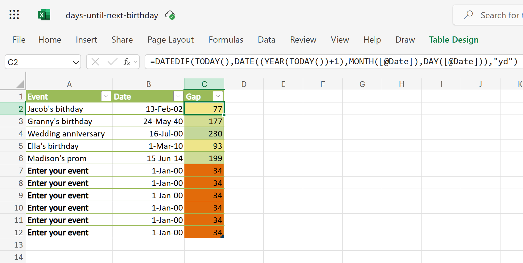
Don't see how this could work for you? Think about it in another way… Suppose you have a list of birthdays of your family members and friends. Would you like to know how many days there are until their next birthday? Moreover, how many days exactly are left until your wedding anniversary and other events you wouldn't want to miss? Easily!
The formula you need is this (where A is your Date column):
=DATEDIF(TODAY(), DATE((YEAR(TODAY())+1), MONTH($A2), DAY($A2)), "yd")
The "yd" interval type at the end of the formula is used to ignore years and calculate the difference between the days only. For the full list of available interval types, look here.
Tip. If you happen to forget or misplace that complex formula, you can use this simple one instead: =365-DATEDIF($A2,TODAY(),"yd"). It produces exactly the same results, just remember to replace 365 with 366 in leap years : )
And now let's create an Excel conditional formatting rule to shade different gaps in different colors. In this case, it makes more sense to utilize Excel Color Scales rather than create a separate rule for each period.
The screenshot below demonstrates the result in Excel - a gradient 3-color scale with tints from green to red through yellow.

"Days Until Next Birthday" Excel Web App
We have created this Excel Web App to show you the above formula in action. Just enter your events in 1st column and change the corresponding dates in the 2nd column to experiment with the result.
If you are curious to know how to create such interactive Excel spreadsheets, check out this article on how to make web-based Excel spreadsheets.
Hopefully, at least one of the Excel conditional formats for dates discussed in this article has proven useful to you. If you are looking for a solution to some different task, you are most welcome to post a comment. Thank you for reading!
758 comments
Hi.
I followed your instructions so I could colour-code for reporting due; within 1 week (red), 2 weeks (orange), 3 weeks (yellow), 30 days (green) and >30 days (blue):
RED: =AND($G3-TODAY()>=0,$G3-TODAY()=8,$G3-TODAY()=15,$G3-TODAY()=22,$G3-TODAY()30
For some reason, cells with the same date are formatted differently. i.e., there are four lines where the date is 11 Feb 2026, but only the first three lines are red, the fourth is orange. Again, there are three lines where the due date is 18 Feb, but the first two are orange and the third is yellow. 5 Marsh is within 30 days (Feb only being 28) but the last 5 march entry is blue instead of green.
How do I ensure my dates are treated consistently?
Hi! I can't verify your formula because I don't know which data range you applied conditional formatting to, and your formula isn't complete. However, these two conditions can't be met simultaneously using the AND condition: $G3-TODAY()=8,$G3-TODAY()=15
I recommend reading this guide: Apply multiple rules to same cells.
I have created a Yearly Calendar for our staff to show holidays at a glance, I have formatted all cells to have colour code for each person to automatic fill. But how do I amend the formatting to show multiple people off on the same day.
Hi! Your information is not enough to understand what problem you are solving and what conditional formatting you want to apply. The information you provided is not enough to understand your case and give you any advice, sorry.
I'm trying to set formatting to color code age ranges and it doesn't seem to be working. Here are my 3 formulas:
=AND($E3-TODAY()>=0, $E3-TODAY()1825, TODAY()-$E3>1095) Shaded Yellow
=TODAY()-$E3>1895 Shaded Red.
These are in the order I pasted them, but only the yellow is showing up and not in the correct date ranges..... Please Help!
Hi! Unfortunately, your formulas are incomplete. There are only two formulas. Perhaps the formula can be corrected as follows:
=AND($E3-TODAY()>=0, $E3-TODAY()<1825, $E3-TODAY()>1095)
Here is the guide that may be helpful to you: Apply multiple rules to same cells.
Thanks Alexander, but there are 3 rules I added. It didn't put them on separate lines as I typed them, so I think you misunderstood. I put the "Color" at the end of each rule to separate them. 1 rule is for greater than 5 years, one is for 3-5 years and the other is for 0-3 years..... Red, Yellow, Green in that order.
Thanks.
I am looking for a formula to add conditional formatting to trigger within 30 days of the due date for a cell.
Example: a certificate expires Mar 8-2026 and I would like to add yellow for within 30 days and any date after 30 red is indicated in the cell.
Thank you in advance
Hello Victoria!
Pay attention to the following paragraph of the article above: How to highlight dates within a date range. The formula might look like this:
=AND((A1-TODAY())<30,TODAY()<A1)
Similarly, create formula for the second condition and use these guidelines: Apply multiple rules to same cells.
Hi, I'm struggling to understand some of this.
I work in a warehouse and use a system similar to this, the formats are the same.
We use expedition times, so trucks that have to be leaving or should've been gone by a certain time
The first column literally says "expeditiontime".
Formulated like this: 30-09-2025 05:12:00.
What format or formula do I use, that an hour and half before this expedition time, it turns yellow. For an hour before, it turns red, and after the expedition time is goes back to white?
I hope I explained this correctly
Hello Melly!
You can get the current date and time using NOW function. Since time is stored as a number in Excel, 1 hour is 1/24.
=A1-NOW()<(1/24*1.5)
Create a separate conditional formatting rule for each condition. For information on how to correctly apply multiple formatting rules to a single cell, see this guide: Apply multiple rules to same cells.
Hi,
I have a list of dates (compliance dates) that have a tolerance of 91 days either side.
How can I create a formula to highlight the cells as dark shaded green when they are 91 before the compliance date to dark shaded red when they are 91 after the compliance date to easily highlight when the dates are past their compliance?
Thanks.
Hi! Read the following paragraph in the article above very carefully: How to highlight dates within a date range. See formula examples and instead of the current date, use an absolute reference to cell with the date you need.
I have investment report where five individuals subscribe per month in excel i would like to use condition formatting to flag any colour when ever the responsible person has delayed to pay his investment contribution
Hi! Without seeing your data, it is impossible to recommend conditional formatting formula. However, you can select all dates that are less than current date using the recommendations described in the article above.
I have conditional formatting that underlines the last day of the month in several columns (using EOMONTH formula). I also have conditional formatting that highlights values outside of a min/max as red. When the file is updated (done sporadically), the user needs to drag down the previous row which has no min/max formatting. However, when I have the EOMONTH conditional formatting active, dragging down the row above does not remove the min/max formatting of the cells, they stay red if outside of the range. If I don't have the EOMONTH conditional formatting, it works as expected and dragging down the row above with no min/max formatting removes the min/max formatting of the cells and they are no longer red. Can anyone help?
Hello Katie!
Dragging down a row copies both values and formatting, including conditional formatting rules.
Also when EOMONTH formatting is active, it may be preserving the min/max rule due to how Excel prioritizes conditional formatting.
Excel evaluates rules in order, and if multiple rules apply to the same cell, the one higher in the list takes precedence unless “Stop If True” is checked.
Read more: Apply multiple conditional formatting rules to same cells.
Check Rule Order.
Go to Home > Conditional Formatting > Manage Rules.
If not, reorder them using the arrows.
Also you can in the Conditional Formatting Rules Manager, check the box for “Stop If True” on the EOMONTH rule.
This prevents Excel from applying further rules if EOMONTH condition is met.
Another way - clear formatting before dragging.
Before dragging down, clear conditional formatting from the destination cells.
Also make sure your formulas use correct referencing. For example:
=$A1=EOMONTH($A1,0) vs =A1=EOMONTH(A1,0)
Incorrect referencing can cause rules to behave unexpectedly when copied. Read more: Relative and absolute cell references in Excel conditional formatting.
Thank you for the info you publish! I'm trying to use conditional formatting to highlight cells that contain dates that are prior to the previous month. I tried =MONTH(F2) < MONTH(TODAY())-1 but this doesn't take into account the year and highlights cells in future years but previous months. I've used the already available this month, last month and next month, but want to easily see those that have been tardy in responding to me from the previous months. Do you have any suggestions please.
Hello Ellie!
To get the last day of the month, you can use EOMONTH function. For example, try this conditional formatting rule:
=F2<=EOMONTH(TODAY(),-2)
I'd like to create a condition for when the date in column A is less than 120 days of the date in column B of the same row.
Hello Tiffany!
If I understand your task correctly, the following tutorial should help: Excel IF statement between two numbers or dates.
Hi all, is it possible to build a formula to calculate the difference between two m/d/yyy h:mm fields that also excludes weekends? I am able to calculate the difference between the two dates/times but I cannot figure out if there is a way to also exclude weekends. I have used networkdays in the past but that was on date only fields.
Thanks
Hello Jenny!
To calculate difference in hours between two dates excluding weekends, try this formula:
=A2-A1-NETWORKDAYS.INTL(A1,A2,"1111100")
You can calculate the number of weekends using the NETWORKDAYS.INTL function.
To correctly show the date difference in hours, use these instructions: How to show over 24 hours, 60 minutes, 60 seconds in Excel.
I am new to excel and need a conditional format for a date. We do training on a certain date, but I want to be able to be notified in yellow when that retraining date is coming up 30 days prior, the retraining is every 3 years.
Hello Lara!
I hope you have studied the recommendations in the tutorial above. It contains answers to your question. Example of conditional formatting formula:
=A1-TODAY()<30
You can also find useful information in this guide: Add years to date in Excel.
HI Good Day to all,
Can you help me with my problem i have almost 100k of my daily observation. Some are Closed and some remain open. i need a formula or conditional formatting that the "open" observation will automatically change to "overdue" after 10 days of date observation (in different column). I've been manually doing that.
Thank you in advance.
Hi! Conditional formatting cannot change value in cell. Try to calculate number of days between current date and date written in cell. Then use IF formula to show one of two values. For example:
=IF(TODAY()-A1>10,"overdue", "open")
You can also use a VBA macro to automatically change value in cell depending on condition being met.
Thanks for the Employee Absence Tracker!
I wonder if it's possible to change the year e.g., our vacation year is December to November. Is there a way of changing this to run December 1st to November 30th every year?
Hello Kay!
You can create any date using the DATE function. You can also automatically subtract month from date using the EDATE function. For example, subtract one month from date:
=EDATE(A1,-1)
I can't give more specific advice as I don't know what you want to do.
I want to highlight a date 2 months in the past. Love the "a date occurring" options, this gives me last month, but I need 2 months ago. Is that possible?
Hello Stacey!
Use the EOMONTH function to set the start and end dates of the interval last 2 months before the current date. Here is an example of a conditional formatting formula for dates in column D.
=AND(D1>EOMONTH(TODAY(),-3),D1<EOMONTH(TODAY(),-1))
I want to conditional format a cell based on a date cell + a number of days. Example: =IF(H34+10<I34, TRUE, FALSE) I have +15 and +20. I then do that for J34, K34, L34, and M34 all off the cell to the left. The formatting works. What I need is that I need to do this for 10+ lines of excel but all need to be independent. e.g. H35, H36, H37 and so on.
When I try to copy and paste, or apply to a range, it keeps the H34 even though it is not formatted $H$34. Is there a way I can cascade my formulas so I don't have to input them each by hand. That is a lot of coding.
Hi! Maybe this guide will be helpful: How to copy Excel conditional formatting.
Hi - In Excel I have a cell which records an altered dollar amount. The date on which this happens is manually written into a cell nearby. It is not a daily event, therefore the date may not change for days or even weeks. I would like to automate the cell carrying the date, so that when the dollar amount changes in one cell, the date changes as well, and stays fixed until the next time the dollar amount changes.
Thanks,
Roger
Hello Roger!
If I understand your task correctly, to prevent your date from automatically changing, you can use several methods:
1. Use Shortcuts to insert the current date and time
2. Use the recommendations How to insert today date & current time as unchangeable time stamp in our blog.
3. Replace the date and time returned by the TODAY function with their values. Copy the date (CTRL + C), then paste only the values using Paste Special or Shortcut CTRL + ALT + V.
4. Use VBA to write the current date and time to the cell.
Good Day All
I want Excel to insert the date in Colum "A" if I insert date in Colum "B"
Many Thanks
Hello Marius!
If you want to show the current date in column B by condition, use the IF formula and TODAY function.
=IF(B1<>"",TODAY(),"")
Set the date format you want in the formula cell as described here: How to change Excel date format and create custom formatting.
If this date should not change, try these instructions: Formula to insert today date & current time as unchangeable time stamp. Or use a VBA macro to insert a date automatically.
Hello,
Can someone help me out with below query in excel how to resolved with functions and formulas
i want to change the date as per status change in one cell by following the various status which are change within 1/2 days
For example: Today i done a booking for part load so i change the status as "booking received" The very next day i am change the status as "Booking Done" and last day means after 3/4 day i change the status as "delivery completed" so every status change i want to record the current date and as status change date should be followed by status change effective date, also if possible i want to check the History of the Cell on which date the status is change Link Google edit history
Hello!
If I understand your task correctly, to insert and prevent date from automatically changing, you can use several methods:
1. Use Shortcuts to insert the current date and time
2. Use the recommendations How to insert today date & current time as unchangeable time stamp in our blog.
3. Replace the date and time returned by the TODAY function with their values. Copy the date (CTRL + C), then paste only the values using Paste Special or Shortcut CTRL + ALT + V.
4. Use VBA to write the current time to the cell.
Hi! I found this post and it goes in a similar direction like the problem i would like to solve.
I'm creating kind of a calendar for a whole year - see screenshot here:
https://drive.google.com/file/d/1O4HaEpp2VS85fsPvQDcqNBmprAMtqVDC/view?usp=sharing
In the screenshot i annotated 2 areas - in the calendar itself (blue) and in a list below the month (red). Both are formatted as dates.
What i would like to do is to highlight a date in the calendar (change it's font color), if there is one or more entries in the list below with the same date.
Is that even possible?
Glad for every direction or help with the formula
Thanks + best regards!
Achim
Hi! Use the DAY function to get the day from the date. Use the SUMPRODUCT function to determine if the day is the same as the numbers on the calendar (blue). Use conditional formatting as recommended in this article: Relative and absolute cell references in Excel conditional formatting.
=SUMPRODUCT(--(D$2=DAY($A$3:$A$16)))>0