Comparing columns in Excel is something that we all do once in a while. Microsoft Excel offers a number of options to compare and match data, but most of them focus on searching in one column. In this tutorial, we will explore several techniques to compare two columns in Excel and find matches and differences between them.
How to compare 2 columns in Excel row-by-row
When you do data analysis in Excel, one of the most frequent tasks is comparing data in each individual row. This task can be done by using the IF function, as demonstrated in the following examples.
Example 1. Compare two columns for matches or differences in the same row
To compare two columns in Excel row-by-row, write a usual IF formula that compares the first two cells. Enter the formula in some other column in the same row, and then copy it down to other cells by dragging the fill handle (a small square in the bottom-right corner of the selected cell). As you do this, the cursor changes to the plus sign:
To find cells within the same row having the same content, A2 and B2 in this example, the formula is as follows: To find cells in the same row with different values, simply replace the equals sign with the non-equality sign (<>): And of course, nothing prevents you from finding both matches and differences with a single formula: Or The result may look similar to this:
As you see, the formula handles numbers, dates, times and text strings equally well. Tip. You can also compare two columns row-by-row using Excel Advanced Filter. Here is an example showing how to filter matches and differences between 2 columns.
Formula for matches
=IF(A2=B2,"Match","")
Formula for differences
=IF(A2<>B2,"No match","")
Matches and differences
=IF(A2=B2,"Match","No match")=IF(A2<>B2,"No match","Match")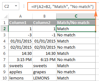
Example 2. Compare two lists for case-sensitive matches in the same row
As you have probably noticed, the formulas from the previous example ignore case when comparing text values, as in row 10 in the screenshot above. If you want to find case-sensitive matches between 2 columns in each row, then use the EXACT function:
=IF(EXACT(A2, B2), "Match", "")
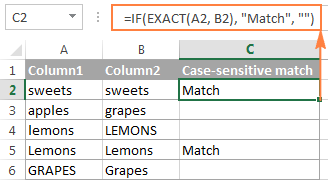
To find case-sensitive differences in the same row, enter the corresponding text ("Unique" in this example) in the 3rd argument of the IF function, e.g.:
=IF(EXACT(A2, B2), "Match", "Unique")
Compare multiple columns for matches in the same row
In your Excel worksheets, multiple columns can be compared based on the following criteria:
- Find rows with the same values in all columns (Example 1)
- Find rows with the same values in any 2 columns (Example 2)
Example 1. Find matches in all cells within the same row
If your table has three or more columns and you want to find rows that have the same values in all cells, an IF formula with an AND statement will work a treat:
=IF(AND(A2=B2, A2=C2), "Full match", "")
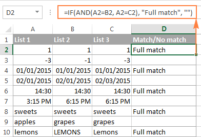
If your table has a lot of columns, a more elegant solution would be using the COUNTIF function:
=IF(COUNTIF($A2:$E2, $A2)=5, "Full match", "")
Where 5 is the number of columns you are comparing.
Example 2. Find matches in any two cells in the same row
If you are looking for a way to compare columns for any two or more cells with the same values within the same row, use an IF formula with an OR statement:
=IF(OR(A2=B2, B2=C2, A2=C2), "Match", "")
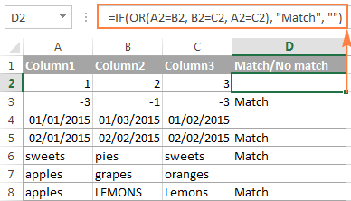
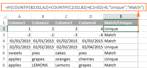
In case there are many columns to compare, your OR statement may grow too big in size. In this case, a better solution would be adding up several COUNTIF functions. The first COUNTIF counts how many columns have the same value as in the 1st column, the second COUNTIF counts how many of the remaining columns are equal to the 2nd column, and so on. If the count is 0, the formula returns "Unique", "Match" otherwise. For example:
=IF(COUNTIF(B2:D2,A2)+COUNTIF(C2:D2,B2)+(C2=D2)=0,"Unique","Match")
How to compare two columns in Excel for matches and differences
Suppose you have 2 lists of data in Excel, and you want to find all values (numbers, dates or text strings) which are in column A but not in column B.
For this, you can embed the COUNTIF($B:$B, $A2)=0 function in IF's logical test and check if it returns zero (no match is found) or any other number (at least 1 match is found).
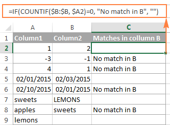
For instance, the following IF/COUNTIF formula searches across the entire column B for the value in cell A2. If no match is found, the formula returns "No match in B", an empty string otherwise:
=IF(COUNTIF($B:$B, $A2)=0, "No match in B", "")
Tip. If your table has a fixed number of rows, you can specify a certain range (e.g. $B2:$B10) rather than the entire column ($B:$B) for the formula to work faster on large data sets.
The same result can be achieved by using an IF formula with the embedded ISERROR and MATCH functions:
=IF(ISERROR(MATCH($A2,$B$2:$B$10,0)),"No match in B","")
Or, by using the following array formula (remember to press Ctrl + Shift + Enter to enter it correctly):
=IF(SUM(--($B$2:$B$10=$A2))=0, " No match in B", "")
If you want a single formula to identify both matches (duplicates) and differences (unique values), put some text for matches in the empty double quotes ("") in any of the above formulas. For example:
=IF(COUNTIF($B:$B, $A2)=0, "No match in B", "Match in B")
How to compare two lists in Excel and pull matches
Sometimes you may need not only match two columns in two different tables, but also pull matching entries from the lookup table. Microsoft Excel provides a special function for this - the VLOOKUP function. As an alternative, you can use a more powerful and versatile INDEX MATCH formula. The users of Excel 2021 and Excel 365, can accomplish the task with the XLOOKUP function.
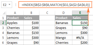
For example, the following formulas compare the product names in columns D against the names in column A and pull a corresponding sales figure from column B if a match is found, otherwise the #N/A error is returned.
=VLOOKUP(D2, $A$2:$B$6, 2, FALSE)
=INDEX($B$2:$B$6, MATCH($D2, $A$2:$A$6, 0))
=XLOOKUP(D2, $A$2:$A$6, $B$2:$B$6)
For more information, please see How to compare two columns using VLOOKUP.
If you don't feel very comfortable with formulas, you can have the job done using a fast and intuitive solution - Merge Tables Wizard.
Compare two lists and highlight matches and differences
When you compare columns in Excel, you may want to "visualize" the items that are present in one column but missing in the other. You can shade such cells in any color of your choosing by using the Excel Conditional Formatting feature and the following examples demonstrate the detailed steps.
Example 1. Highlight matches and differences in each row
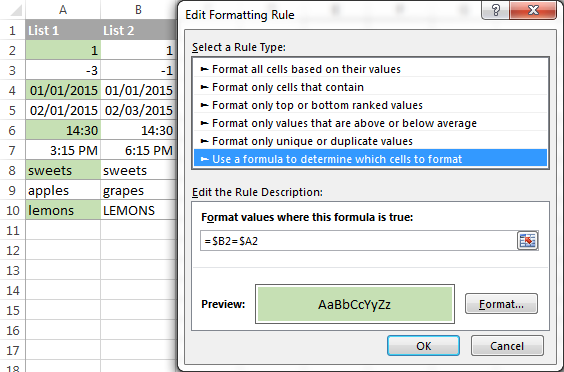
To compare two columns and Excel and highlight cells in column A that have identical entries in column B in the same row, do the following:
- Select the cells you want to highlight (you can select cells within one column or in several columns if you want to color entire rows).
- Click Conditional formatting > New Rule… > Use a formula to determine which cells to format.
- Create a rule with a simple formula like
=$B2=$A2(assuming that row 2 is the first row with data, not including the column header). Please double check that you use a relative row reference (without the $ sign) like in the formula above.
To highlight differences between column A and B, create a rule with this formula:
=$B2<>$A2
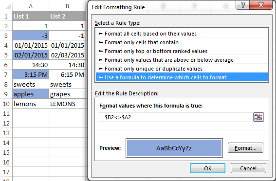
If you are new to Excel conditional formatting, please see How to create a formula-based conditional formatting rule for step-by-step instructions.
Example 2. Highlight unique entries in each list
Whenever you are comparing two lists in Excel, there are 3 item types that you can highlight:
- Items that are only in the 1st list (unique)
- Items that are only in the 2nd list (unique)
- Items that are in both lists (duplicates) - demonstrated in the next example.
This example demonstrates how to color the items that are only in one list.
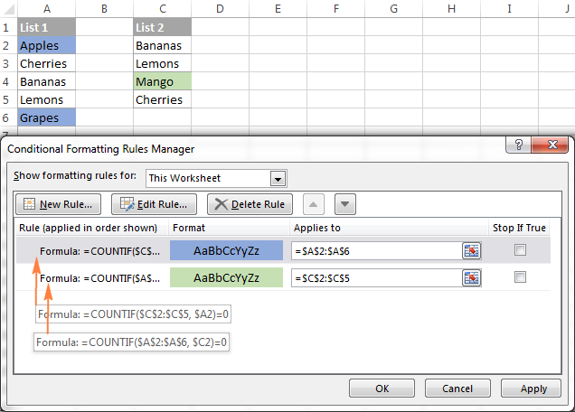
Supposing your List 1 is in column A (A2:A6) and List 2 in column C (C2:C5). You create the conditional formatting rules with the following formulas:
Highlight unique values in List 1 (column A):
=COUNTIF($C$2:$C$5, $A2)=0
Highlight unique values in List 2 (column C):
=COUNTIF($A$2:$A$6, $C2)=0
And get the following result:
Example 3. Highlight matches (duplicates) between 2 columns
If you closely followed the previous example, you won't have difficulties adjusting the COUNTIF formulas so that they find the matches rather than differences. All you have to do is to set the count greater than zero:
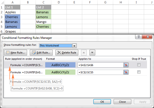
Highlight matches in List 1 (column A):
=COUNTIF($C$2:$C$5, $A2)>0
Highlight matches in List 2 (column C):
=COUNTIF($A$2:$A$6, $C2)>0
Highlight row differences and matches in multiple columns
When comparing values in several columns row-by-row, the quickest way to highlight matches is creating a conditional formatting rule, and the fastest way to shade differences is embracing the Go To Special feature, as demonstrated in the following examples.
Example 1. Compare multiple columns and highlight row matches
To highlight rows that have identical values in all columns, create a conditional formatting rule based on one of the following formulas:
=AND($A2=$B2, $A2=$C2)
or
=COUNTIF($A2:$C2, $A2)=3
Where A2, B2 and C2 are the top-most cells and 3 is the number of columns to compare.
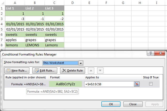
Of course, neither AND nor COUNTIF formula is limited to comparing only 3 columns, you can use similar formulas to highlight rows with the same values in 4, 5, 6 or more columns.
Example 2. Compare multiple columns and highlight row differences
To quickly highlight cells with different values in each individual row, you can use Excel's Go To Special feature.
- Select the range of cells you want to compare. In this example, I've selected cells A2 to C8.

By default, the top-most cell of the selected range is the active cell, and the cells from the other selected columns in the same row will be compared to that cell. As you can see in the screenshot above, the active cell is white while all other cells of the selected range are highlighted. In this example, the active cell is A2, so the comparison column is column A.
To change the comparison column, use either the Tab key to navigate through selected cells from left to right, or the Enter key to move from top to bottom.
Tip. To select non-adjacent columns, select the first column, press and hold Ctrl, and then select the other columns. The active cell will be in the last column (or in the last block of adjacent columns). To change the comparison column, use the Tab or Enter key as described above.
- On the Home tab, go to Editing group, and click Find & Select > Go To Special… Then select Row differences and click the OK button.
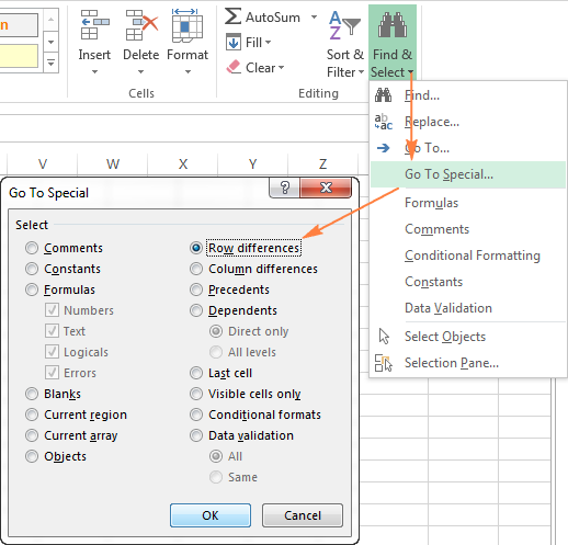
- The cells whose values are different from the comparison cell in each row are colored. If you want to shade the highlighted cells in some color, simply click the Fill Color icon on the ribbon and select the color of your choosing.

How to compare two cells in Excel
In fact, comparing 2 cells is a particular case of comparing two columns in Excel row-by-row except that you don't have to copy the formulas down to other cells in the column.
For example, to compare cells A1 and C1, you can use the following formulas.
For matches:
=IF(A1=C1, "Match", "")
For differences:
=IF(A1<>C1, "Difference", "")
To learn a few other ways to compare cells in Excel, please see:
Formula-free way to compare two columns / lists in Excel
Now that you know Excel's offerings for comparing and matching columns, let me show you our own solution for this task. This tool is named Compare Two Tables and it is included in our Ultimate Suite.
The add-in can compare two tables or lists by any number of columns and both identify matches/differences (as we did with formulas) and highlight them (as we did with conditional formatting).
For the purpose of this article, we'll be comparing the following 2 lists to find common values that are present in both.

To compare two lists, here are the steps you need to follow:
- Start with clicking the Compare Tables button on the Ablebits Data tab.

- Select the first column/list and click Next. In terms of the add-in, this is your Table 1.

- Select the second column/list and click Next. In terms of the add-in, it is your Table 2, and it can reside in the same or different worksheet or even in another workbook.

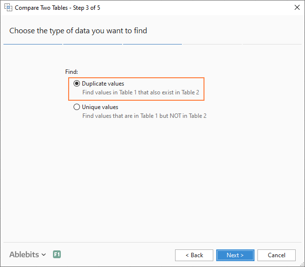
- Choose what kind of data to look for:
- Duplicate values (matches) - the items that exist in both lists.
- Unique values (differences) - the items that are present in list 1, but not in list 2.
Since our aim is to find matches, we select the first option and click Next.
- This is the key step where you select the columns for comparison. In our case, the choice is obvious as we are only comparing 2 columns: 2000 Winners against 2021 Winners. In bigger tables, you can select several column pairs to compare by.

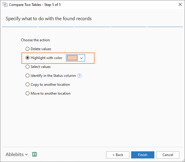
- In the final step, you choose how to deal with the found items and click Finish.
A few different options are available here. For our purposes, these two are most useful:
- Highlight with color - shades matches or differences in the selected color (like Excel conditional formatting does).
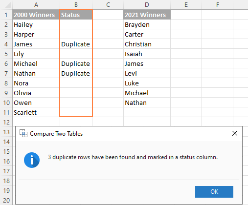
- Identify in the Status column - inserts the Status column with the "Duplicate" or "Unique" labels (like IF formulas do).
For this example, I've decided to highlight duplicates in the following color:
And in a moment, got the following result:

With the Status column, the result would look as follows:
Tip. If the lists you are comparing are in different worksheets or workbooks, it might be helpful to view Excel sheets side by side.
This is how you compare columns in Excel for matches (duplicates) and differences (unique values). If you are interested to try this tool, you are welcome to download an evaluation version using the below link.
I thank you for reading and encourage you to check out other helpful tutorials that we have :)
Available downloads
Compare Excel Lists - examples (.xlsx file)
Ultimate Suite - trial version (.exe file)
 by
by
546 comments
i have details in two columns as origin and destiantion ---- in same record some locations which are in destination are avbl as origin too...now i want both those location together which are having similar name irrespective of origin or dest...
COLM A COLUM B SALE
ORG DEST.
DELHI GURGAON 15
INDORE BHOPAL 20
GURGAON DELHI 18
NOW HOW CAN I GET COMMON LOCATION (DELHI-GURGAON & GURGAON-DELHI)ALTOGETHER ----OR INFRONT OF
EACHOTHER.
I have two columns in a worksheet, column one is a share code (300 codes) column two is that share capitalization in greater to smaller order. These two columns are only entered once a year at the beginning of the financial year.
Column 3 and 4 are entered once a week and formatted in the same way greater to smaller but course the order will be different as capitalization change.
so for example row 1 in column A will show a code for the highest capitalization at the beginning of the year.
but one month later column 3 and four will show a different result.
I would like to high light these change by colour change in the positive changes only row cells.
Hi I want to extract a text which is not matching with other text in two columns. is there any formula we can use in excel
Conditional Formatting 'Add Rule' does not appear on Excel Online. Can someone kindly advise how to set up formatting which highlights a cell when that cell matches any given number in a table range?
The 'equal to' option only seems to work for cell to cell value. I would like to search a table and the result would be Green for 'match' and red for 'no match' value.
DATE PRODUCT OPEING STOCK IN OUT RETURN CLOSING
01-06-19 A 100 10 5 20 125
01-06-19 B 200 20 10 30 240
02-06-19 A 125
02-06-19 B 240
NEW DATE ENTER TO CLOSING STOCKING AUTOMATIC OPENING STOCK & ONE DATE ENTER TO ALL ONE DATE PRODUCT SHOW FORMULA
I think you meant well, but your explanation is confusing to me. Sorry.
Thnakyou. Loads of love and gratitude.
Dear all,
Anyone know how to get ride of the #N/A form the formula of INDEX($B$33,MATCH(B5,$B$33,0),1).
In fact, i just want a "" if not match.
Thank you.
Hello,
I would like to seek your support in the below, i have a long list of Part numbers in column A (one part number could be repeated in different rows) and the unit price in Column B. I need a formula so i can know if the same part number has different Unit prices.
Thanks
Hi
I have an issue with excel. I have 3 columns. 1 column having a series and 1 column having a list and another one having a subset of the column having the list. If the subset has the value present in the list mentioned in the main list, need to replace it with the equivalent from the series list beside the main list.
Kindly support
Hi there
I have a large Excel file with 3 Columns and consists of cross references.
There are instances where duplications do occur but it depends on if both columns match.
As an example this would be valid because it relates two different parts
PART01 - XREF01
PART02 - XREF01
But I want to get rid of instances where two rows match in both columns:
PART01 - XREF01
PART01 - XREF01
Any help and guidance would be very much appreciated.
Thanks and Best Regards
Steve
I want a formula to identify if a particular customer code is allocated to more than two customers. For example, there are two customers A & B each having a respective customer code as A1 & B1 respectively, if by any chance the A1 code is allocated to customer B, then the cell should reflect an error.
find difference of D and E column , even we add new column before D
I need to compare 3 columns in which the three columns contain certain different values ie., 1,2,3 which match corresponding values in the same row. Also the matching values are not in the same row. Also i wish to highlight the cells with matching values.
=IF(AND(A2=1,C2=1),"1"),IF(AND(B3-C3=1),A3=2,"2"),IF(AND(A4=B4=2),C4=1,"3"),IF(AND(A5=1,C5=2),"4"),IF(AND(A6=C6=2),B6=1,"5"),IF(AND(A7=2,B7=2,C7=2),"6")
please help the correct sintex in the above formula and send my mail, thanks
Good Day Team
Now on the right hand side you have the 0's and 1's, which is what i want Excel to fill appropriately.
On the left hand is that data source
Now it should work like this:
Check H3 within B3:G4
If found use '1' if not found use '0'
Now rightly O4 worked appropriately by detecting "Guilder" in A4 and "Guilder" in O4 returning '1' and same for "Guinness stout"
But for Hero it returned "0", which is wrong.
Please i want to code appropriately by telling excel to search for entries in row 3 as reference from A4:F4.
For instance, Search for "33 Export" in H3 within the array A4:F4, if True return 1, else return 0. do this for all other products till you get to "Hero". Next Repeat same process in other rows downwards retaining H3:S3 as a fixed reference.
Can you help?
Thanks so much i await your response
hi
I need to compare 2 columns in which both columns contain certain matching text which match corresponding amounts in the same row. Also the matching text are not in the same row. Also i wish to highlight the cells with matching texts.
is there a formula?
Helo. I have a problem. The problem is that I have a master list of two pages comprising of three columns i.e Economic Class, ID code and Activity. Now every month I have to extract a list of 30 pages in excel and verify if there has been any wrong combinations in connection with my master list. I would be very grateful if I could be shown a way of how to do it using a formula.
Thank you.
Hello,
I am trying to reconcile inventory data. I have a list of asset ID's in column A pulled from a database export. Their database location is in column B.
I want to make sure my scanned Asset ID's and Locations Match what is in the database (or highlight when they don't match so I can make a movement in the database)
My plan was to add the scanned asset tag data below the asset ID's in column A and the associated scanned locations in column B. I highlight duplicates from column A to make sure I accounted for all of them. Is there a way to say "IF column A has a duplicate value in another row further down the spreadsheet, does column B match the row?"
Essentially I want it to find the duplicate data in the same column and then make sure column B also matches for that duplicate.
I might be making this harder than it has to be, just couldn't find a good way to organize that formula.
Hello, I have two columns, say column A and column B, with pricing in them and I want to compare those. I want to highlight the value in column B if it is + or - 10% of the value in column A. Looking for the formula I should use to get there. Thanks
Hi,
Below is the data,
Sale order have a some of line items and result is three type A, B, C
For one sale order all line item has C means , result should come as Completed
Sale Order # Line # Status
10045 10 A
10048 20 C
10045 30 C
10045 40 C
10045 50 B
10045 60 C
10046 10 C
10046 20 C
10046 30 C
10046 40 C
10046 50 C
10046 60 C
=IF((P2=L:L),IF(N:N="C","Completed","Not Completed"))
Pls confirm
Saran:
If I understand your question this should work:
=IF(C2="C"',"Completed","Not Completed")
Then just copy the formula down the column to get the results for the respective data. No need to enter a range as in "L:L".
Hello..I have two sheet in first sheet 5 columns like gstin no., invoice no., amount, cgst, and sgst in second sheet also same columns there are more data. Now i want to find match firts sheet data in second sheet is it possible to find match data in easy method and short time please tell me.
Hello! I have a situation where for two columns (product number and colour), if any rows in first column (Product Number) have duplicate values, then the corresponding value of colour (second column) SHOULD also be the the same. If there are any violations, then they must be highlighted.
Example:
Product Number Colour
12345678 Black
12345678 Black
12986533 Blue
12344321 Red
12344321 Yellow
In above example, row 1 and 2 must pass the condition (duplicate values in both columns) but row 3 and 4 must fail and must be highlighted (duplicate values in one columns but not in another).
Expected result
* Rows in column 1 with no duplicates be ignored
* Rows with duplicates in column 1 and also in column 2 be ignored
* Rows with duplicates in column 1 but not in column 2 must be highlighted
In above examples, rows to be highlighted are
12344321 Red
12344321 Yellow
Thanks!
Thanks so much for this tutorial. I've read each response but still haven't found the solution I need. How can I perform a case insensitive partial match from one column to the next? Example.
Column A
green
red
brown
Column B
The green tree
Orange Leaves
Brown Dirt
I would like to search all the phrases in Column B with the words in Column A.
Desired Outcome:
The Phrase "The green tree" in column B should be identified because the word "green" from column A was found.
The Phrase "Brown Dirt" in column B should be identified because the word "brown" from column A was found.
I've scoured the web looking for a solution and I haven't found one that can be easily used without the knowledge of writing code.
Have you been able to find a solution for this? I have the exact same issue. I only need to find a partial match and then sum it all up. I have over 80k (x3) line items to search...
This post was SO helpful thank you!
Thank You
Sorry you are having problems. Here is a copy of my IF(Countif ..... formula and this should help you, I hope.
=IF(COUNTIF('2017 Assigned Org'!$A$5:$A$70,'2018 Assigned Org'!A7)=0,"New RC","")
In my example, I am trying to find new RC's that were added in 2018 but did not exist in 2017. So my formula checks if the value in cell A7 of the 'Assigned Org' worksheet is found in rows A5:A70 of the '2017 Assigned Org' worksheet. And, I copy down the formula to all the rows in my '2018 Assigned Org' worksheet.
Hi all,
I tried the countif >0 formula to highlight duplicates in 2 different columns, I don't know whether I did it wrong.
I have about 1500 cells in the one column (A) with invoice numbers, then in another column(B) are fewer invoice numbers that have been selected from the invoice numbers in (A). As a sample.
I now want to go an highlight the invoice numbers that have been selected in B, in A, but quickly.
PLEASE help. I really don't want to have to scroll through or even ctrl+f.
Thank you
L
Thanks for the information, that really very much helpful.
This helped so much!!!!!!!!!!!!!!!!!!!!! THANK YOU!
Nimsoft Dynatrace Match/No Match
ATG BAU-API
I'm not able to sort by the matchs. Even tried =IF(B3=C3, "Match", "")
could you please help me.
Example four does not do what you say. It does not compare two columns. It compares all cells in the columns; therefore, it will highlight all duplicates even if they are in the same column.
Hi Doug,
You are absolutely right. Don't know what I was thinking. I have removed that example from the article. Thank you for pointing that out!
Hello,
Hope you are all well. How to compare sheet1 to sheet2 and both have five columns in each UniqueId, FName, LName, MName, Status in Excel. First it should consider unique id, once UniqueId matches then it needs to make sure the other columns are matching exactly as other columns based on UniqueId. If they are not matching it should say False. I would appreciate if you could help me out
Thanks for your great work you do by helping others..
I have a unique problem seeking formula for use in Office 2010.
Problem: Looking for a formula to :- Find matches in any two cells in the same row where.. For example column A has exactly five or 8 digit numbers and column B has only a single digit with result in column c stating match/no match
Say.. i have two columns in Excel each having numbers.In the first column A i have 5 or 8 number digits exactly. in B i have a single digit. what i need to do is find if the number present in column B, is matching in column A with result in column c stating match/no match i have enjoyed your formula given "Example 2. Find matches in any two cells in the same row
If you are looking for a way to compare columns for any two or more cells with the same values within the same row, use an IF formula with an OR statement: =IF(OR(A2=B2, B2=C2, A2=C2), "Match", "") " ...... But not helping with my problem Please reply. thanks
I guess vlookup has the capability to see if element in column B is present in column A by comparing it with the whole column A. I have done it and am not able to figure out how to do it. Can you tell it.
What if I need to mark a duplicate ONLY if the data in two columns is the same as in a different row?
batch sn
784666 F00001 S006
784664 F00001 S005
784668 F00001 S005
784668 F00001 S006
784668 F00001 S006
Only the bottom row in this sample should be marked as a duplicate....
Hi I am trying to compare twho list and use the formula =countif() but when I write the formula it gives an error that says "there is a problem in formula Not trying to type a formula? ..."
And it does not accept the formula unless I delete = from the formula and if I delete it does not highlight the data. How can I fix it?
Hello. I have a problem. I have been given a spreadsheet of students expected and actual grades in different subjects.
I need to format the data so that if the expected grade is higher than the actual grade both turn red. if the actual grade is higher than the expected grade they both turn green and if both grades are the same they turn yellow.
never mind. I found a solution that works
I have a list of items and all have distinct names. I need to compare the items with a list of known partial matches and have the result be the partial match. For example:
Distinct list:
F-daniel-01
R-rose-20
C-daniel-03
T-bob-35
A-kevin-36
Partial match list:
daniel
rose
bob
kevin
Result:
F-daniel-01 | daniel
R-rose-20 | rose
C-daniel-03 | daniel
T-bob-35 | bob
A-kevin-36 | kevin
Any advise would be great
I have the exact same problem and so far I have not been able to find a solution.
How to give a different mark to Blank cell
=IF(H38645=I38645,"Match","Null")
AA AA
CC CC
TT AA
TT
TT GT
Prices in different location as below :
Article Code - Location A - Location B - Location C - Location D
--------------------------------------------------------------------
GWC-20100 -------- 0 ----------- 0 -------- 43.94 -------- 0 --------
HED-20102 ---------0 --------- 53.55 ---------0 ---------- 0 --------
AFC-201108 --------0 --------- 88.02 ------ 80.02 -------- 0 --------
QRH-201202 --------0 --------- 87.07 -------- 0 -------- 87.07 ------
DJS-201209 ----- 63.09 --------- 0 -------- 63.09 ------ 63.09 ------
HTC-201210 ----- 74.17 ------- 74.17 -------- 0 ---------- 0 --------
PIL-201301 ----- 71.66 ------- 71.66 ------ 71.66 -------- 0 --------
YPC-201305 ----- 70.57 --------- 0 -------- 70.57 -------- 0 --------
RPT-P8157 ------ 51.96 --------- 0 -------- 51.96 ------ 51.96 ------
POL-P9142 -------- 0 ----------- 0 ---------- 0 -------- 36.49 ------
May I know for the above conditions, what are the formula that can be used to cross check whether or not if the article code is having the same price in different location?
Your advise is highly appreciated.
Article Price in Price in Price in Price in
Code Location A Location B Location C Location D
--------------------------------------------------------------------
GWC-20100 43.94
HED-20102 53.55
AFC-201108 80.02 80.02
QRH-201202 87.07 87.07
DJS-201209 63.09 63.09 63.09
HTC-201210 74.17 74.17
PIL-201301 71.66 71.66 71.66
YPC-201305 70.57 70.57
RPT-P8157 51.96 51.96 51.96
POL-P9142 36.49
May I know for the above conditions, what are the formula that can be used to cross check whether or not if the article code is having the same price in different location?
Your advise is highly appreciated.
How to verify if the names in col A have a match in col B using one, or two words contains or any idea how can be done. Thank you
COLUMN A COLUMN B
ANGEL MARIE DIZON ANGEL MARIE E DIZON
OSCAR LUCAS MARK LUCAS MARK OSCAR
JULIE LIM MAN AREVALO
REYNOLD B WILLIAMS JULIE ANN LIM
JEN MARIE YU REYNOLD WILLIAMS
MAN AREVALO B JEN YU
STARK JOHNSON ARCH MAY TAN
ARCH TAN JOHNSON STARK
Jejemole:
I think the only way Excel can be used to help you with this is to use the Fuzzy Logic add-in from Microsoft.
If you Google MS Fuzzy Logic you'll see the address. The description and instructions are there, too.
I have Excel file. Where there were 3 column
1 date
2 credit
3 multiple debit
and I have to reconcile credit debit column and find out difference..
Please help
I have two excel files that have very similar data. I have been using conditional formatting to compare one file to another and to highlight the differences. The issue I am having is that the first column which has the unique value that aligns the rows changes at time. Is there a way to use vlookup to align the rows to then compare for differences so I can highlight the differences?
Hi, I want to compare two lists using excel, but I am not sure how to make it work.
For example,
List 1 contain Apple1234, OrangeXYZ, Banana098, 512Pineapple.
List 2 contain MN_Orange, 3462Apple, 534Pineapple, 786Banana.
I want to arrange List 2 to be same as List 1 based on the fruits, which method should I use?
hello I have a situation where column A contain the staff no. and column B,C,D and E contain Normal hrs.,OT1,OT2, public holiday/sunday hrs.
Now the situation is that I have to cope the B,C,D and E on the same column according to column A (staff no.).
I have two sets of data. Guest by country and I need to copy the same to different sheet.
when excel worksheets have been programmed using these conditions, can we found back the corresponding vba code associated?
J-Law:
In the Developers Tab there is a tool to View Code. When you select it the modules are available. There you can select the module and you'll see the code.
If you don't have the Developers tab active, in 2016 you can see how to open it and how to use the tools in Excel by entering: "Display the relationships between formulas and cells" in the Tell me what you want to do box and click the help option.
Then you'll see the article which addresses your question.
I am a beginner in VBA. i need to compare the values in co11 of row1, row2, row3 so on till the end of the file. if r1c1 = r2c1 then i want to add the values in r1f1 and r2f1, if not equals go to next row. if the value in b1 of row1, row2 and row3 are equal then i wish to add the value of col f in all the rows.
please guide me Ms svet
Prasad:
Assisting users with VBA questions is beyond the scope of this blog. There are many other sites that can help you. Google "Beginner VBA Help" and you will find them.