 by
by In this article, you will find two quick ways to change the background color of cells based on value in Excel 2016, 2013 and 2010. Also, you will learn how to use Excel formulas to change the color of blank cells or cells with formula errors.
Everyone knows that changing the background color of a single cell or a range of data in Excel is easy as clicking the Fill color ![]() button . But what if you want to change the background color of all cells with a certain value? Moreover, what if you want the background color to change automatically along with the cell value's changes? Further in this article you will find answers to these questions and learn a couple of useful tips that will help you choose the right method for each particular task.
button . But what if you want to change the background color of all cells with a certain value? Moreover, what if you want the background color to change automatically along with the cell value's changes? Further in this article you will find answers to these questions and learn a couple of useful tips that will help you choose the right method for each particular task.
How to change a cell's color based on value in Excel dynamically
The background color will change dependent on the cell's value.
Task: You have a table or range of data, and you want to change the background color of cells based on cell values. Also, you want the color to change dynamically reflecting the data changes.
Solution: You need to use Excel conditional formatting to highlight the values greater than X, less than Y or between X and Y.
Suppose you have a list of gasoline prices in different states and you want the prices greater than USD 3.7 to be of the color red and equal to or less than USD 3.45 to be of the color green.

Note: The screenshots for this example were captured in Excel 2010, however the buttons, dialogs and settings are the same or nearly the same in Excel 2016 and Excel 2013.
Okay, here is what you do step-by-step:
- Select the table or range where you want to change the background color of cells. In this example, we've selected $B$2:$H$10 (the column names and the first column listing the state names are excluded from the selection).
- Navigate to the Home tab, Styles group, and choose Conditional Formatting > New Rule….

- In the New Formatting Rule dialog box, select "Format only cells that contain" under "Select a Rule Type" box in the upper part of the dialog box.
- In the lower part of the dialog box under "Format Only Cells with section", set the rule conditions. We choose to format only cells with a Cell Value - greater than - 3.7, as you can see in the screenshot below.

Then click the Format… button to choose what background color to apply when the above condition is met.
- In the Format Cells dialog box, switch to the Fill tab and select the color of your choice, the reddish color in our case, and click OK.

- Now you are back to the New Formatting Rule window and the preview of your format changes is displayed in the Preview box. If everything is Okay, click the OK button.

The result of your formatting will look similar to this:

Since we need to apply one more condition, i.e. change the background of cells with values equal to or less than 3.45 to the green color, click the New Rule button again and repeat steps 3 - 6 setting the required condition. Here is the Preview of our second conditional formatting rule:
When you are done, click the OK button. What you have now is a nicely formatted table that lets you see the highest and lowest gas prices across different states at a glance. Lucky they are in Texas :)

Tip: You can use the same method to change the font color based on the cell's value. To do this, simply switch to the Font tab in the Format Cells dialog box that we discussed in step 5 and choose your preferred font color.


How to permanently change a cell's color based on its current value
Once set, the background color will not change no matter how the cell's contents might change in the future.
Task: You want to color a cell based on its current value and wish the background color to remain the same even when the cell value's changes.
Solution: Find all cells with a certain value or values using Excel's Find All function or Select Special Cells add-in, and then change the format of found cells using the Format Cells feature.
This is one of those rare tasks that are not covered in Excel help files, forums and blogs and for which there is no straightforward solution. And this is understandable, because this task is not typical. And still, if you need to change the background color of cells statically i.e. once and forever unless you change it manually again, proceed with the following steps.
Find and select all cells that meet a certain condition
There may be several possible scenarios depending on what kind of values you are looking for.
If you need to color cells with a particular value, e.g. 50, 100 or 3.4, go to the Home tab, Editing group, and click Find Select > Find….

Enter the needed values and click the Find All button.

Tip: Click the Options button in the right-hand part of the Find and Replace dialog to get a number of advanced search options, such as "Match Case" and "Match entire cell content". You can use wildcard characters, such as an asterisk (*) to find any string of characters or a question mark (?) to find any single character.
In our previous example, if we needed to find all gas prices between 3.7 and 3.799, we would specify the following search criteria:

Now select any of the found items in the lower part of the Find and Replace dialog window by clicking on it and then press Ctrl + A to select all found entries. After that click the Close button.

This is how you select all cells with a certain value(s) using the Find All function in Excel.
However, what we actually need is to find all gas prices higher than 3.7 and regrettably Excel's Find and Replace dialog does not allow for such things.
Luckily, there is another tool that can handle such complex conditions. The Select Special Cells add-in lets you find all values in a specified range, e.g. between -1 and 45, get the maximum / minimum value in a column, row or range, find cells by font color, fill color and much more.

You click the Select by Value button on the ribbon and then specify your search criteria on the add-in's pane, in our example we are looking for values greater than 3.7. Click the Select button and in a second you will have a result like this:

If you are interested to try the Select Special Cells add-in, you can download an evaluation version here.
Change the background color of selected cells using "Format Cells" dialog
Now that all cells with a specified value or values are selected (either by using Excel's Find and Replace or Select Special Cells add-in) what is left for you to do is force the background color of selected cells to change when a value changes.
Open the Format Cells dialog by pressing Ctrl + 1 (you can also right click any of selected cells and choose "Format Cells…" from the pop-up menu, or go to Home tab > Cells group > Format > Format Cells…) and make all format changes you want. We will choose to change the background color in orange this time, just for a change :)

If you want to alter the background color only without any other format changes, then you can simply click the Fill color button and choose the color to your liking.

Here is the result of our format changes in Excel:

Unlike the previous technique with conditional formatting, the background color set in this way will never change again without your notice, no matter how the values change.
Change background color for special cells (blanks, with formula errors)
Like in the previous example, you can change the background color of special cells in two ways, dynamically and statically.
Use Excel formula to change background color of special cells
A cell's color will change automatically based on the cell's value.
This method provides a solution that you will most likely need in 99% of cases, i.e. the background color of cells will change according to the conditions you set.
We are going to use the gas prices table again as an example, but this time a couple of more states are included and some cells are empty. See how you can detect those blank cells and change their background color.
- On the Home tab, in the Styles group, click Conditional Formatting > New Rule… (see step 2 of How to dynamically change a cell color based on value for step-by-step guidance).
- In the "New Formatting Rule" dialog, select the option "Use a formula to determine which cells to format". Then enter one of the following formulas in the "Format values where this formula is true" field:
- =IsBlank()- to change the background color of blank cells.
- =IsError() - to change the background color of cells with formulas that return errors.
Since we are interested in changing the color of empty cells, enter the formula =IsBlank(), then place the cursor between parentheses and click the Collapse Dialog button
 in the right-hand part of the window to select a range of cells, or you can type the range manually, e.g.
 =IsBlank(B2:H12).
- Click the Format… button and choose the needed background color on the Fill tab (for detailed instructions, see step 5 of "How to dynamically change a cell color based on value") and then click OK.
The preview of your conditional formatting rule will look similar to this:

- If you are happy with the color, click the OK button and you'll see the changes immediately applied to your table.


Change the background color of special cells statically
Once changed, the background color will remain the same, regardless of the cell values' changes.
If you want to change the color of blank cells or cells with formula errors permanently, follow this way.
- Select your table or a range and press F5 to open the "Go To" dialog, and then click the "Special…" button.

- In the "Go to Special" dialog box, check the Blanks radio button to select all empty cells.

If you want to highlight cells containing formulas with errors, choose Formulas > Errors. As you can see in the screenshot above, a handful of other options are available to you.
- And finally, change the background of selected cells, or make any other format customizations using the "Format Cells" dialog as described in Changing the background of selected cells.


Just remember that formatting changes made in this way will persist even if your blank cells get filled with data or formula errors are corrected. Of course, it's hard to imagine off the top of the head why someone may want to have it this way, may be just for historical purposes :)
How to get most of Excel and make challenging tasks easy
As an active user of Microsoft Excel, you know that it has plenty of features. Some of them we know and love, others are a complete mystery for an average user and various blogs, including this one, are trying to shed at least some light on them. But! There are a few very common tasks that all of us have to perform daily and Excel simply does not provide any features or tools to automate them or make an inch easier.
For example, if you need to check 2 worksheets for duplicates or merge rows from single or different spreadsheets, it would take a bunch of arcane formulas or macros and still there is no guarantee you would get the accurate results.
That was the reason why a team of our best Excel developers designed and created 70+ add-ins that we call the Ultimate Suite for Excel. These smart tools handle the most grueling, painstaking and error-prone tasks in Excel and ensure quickly, neatly and flawless results. Below is a short list of just some of the tasks the add-ins can help you with:
- Remove duplicates and find unique values
- Merge tables and combine data from different sources
- Combine duplicate rows into one
- Merge cells, rows and columns
- Find and replacing in all data, in all workbooks
- Generate random numbers, passwords and custom lists
- And much, much more.
Just try these add-ins and you will see that your Excel productivity will increase up to 50%, at the very least!
That's all for now. In my next article we will continue to explore this topic further and you will see how you can quickly change the background color of a row based on a cell value. Hope to see you on our blog next week!
73 comments
When
Value of column A Less then Value of column B then column B red
How to create this Formul in excel
Hi! Please read the above article carefully. Also, this article will be helpful: Excel conditional formatting formulas based on another cell.
How do I set the conditional formatting for a drop-down list in order to change background colour whenever I chose a cell value within a selceted range. e.g. I have a list of names from one category (all employees of company A) and another list of names (all employees of comany B). All those names appear in the drop down list but I want to assign green color for all employees from company A and red color for all employees from company B.
Appreciate you help!
Unfortunately, conditional formatting for the drop-down list in Excel is not possible.
you can able to change it using format cells that only contain option
Hi! You can change the font color using the format option for numeric values only. Read more here: Change font color with custom number format. You can apply formatting to cell values, but not to the values shown in the drop down list.
To separate the values in a drop-down list by condition, you can use dependent drop down lists.
How do you apply a =cell<cell logic across a large data set?
Example: I want to conditional format each cell to compare to the same cell in another set of data on the same sheet. The format cell should be red.
E3 needs to compare to U3
E4 needs to compare to U4
F3 needs to compare to V3
F4 needs to compare to V4
G3 needs to compare to X3
G4 needs to compare to X4
Hi!
Select the range of cells you want to highlight with color and create a conditional formatting rule as described in these instructions: Conditional formatting formulas to compare values (numbers and text).
I have prepared a sticker format in excel and returned value using lookup function to fill the sticker details. In one of the cell the value returned shows the category (Color) of the sticker (eg: Purple) , I wanted to change the whole sticker (meaning, the complete sticker range) color according to the color of the value returned (here, Purple). is this possible?
Hi!
You can change the color of a cell by the name of the color that is written in another cell using a VBA macro.
Also, you can use conditional formatting by formula
A1="Purple"
Based on this condition, create a conditional formatting rule with the desired color. For each of the possible colors, create a separate formatting rule.
Hi, how can i change the fill color by using formula for the below
IF my Cell no F16 is X i want to fill entire row 16 as one specific color
can any one help
Hi!
Please have a look at this article — How to change the row color based on a cell's value.
I hope it’ll be helpful.
Hi there,
my problem is a bit different. I want to highlight updated cells in a pre filled data. E.g. I already have a set of data, but due to some reason any one or few cells with existing data may get modified (by someone else in my team), I want to apply conditional formatting to my sheet so that those updated cells get highlighted by its own. So that, next time when I look into my data, it will show me the changes.
Hello!
The Excel formula cannot determine the date the cell was modified. Therefore, conditional formatting using a formula is not possible. Perhaps this article will be useful to you - How to track changes in Excel.
How i can using condition formating if we need notif colour red if im done working 6 day. Every working 6 day automatically red colour
Hello!
Use the NETWORKDAYS function to count the number of business days with slow dates. Read more in this article.
Hi,
What if you wanted the colour to change where the condition is compared to another cell? I want a cell to turn red when the value is less than the other cell, or green if the value is higher.
Hello!
You can learn more about coditional formatting in Excel in this article on our blog — How to use conditional formatting in Excel
It contains answers to your question.
Hi,
Can't find anything on web to help me out with my problem so maybe you can give a hand on this one:
So, I want to create a drop down list with colors (cells with colors so I can chose the color from a list) but I cannot find how to do it. Then I have another one related to the previous which is I want to do a drop down list based on another one but then have the result color based on the text selected from the drop down menu if that makes sense :D... would be very appreciated if someone can help me with it... cheers
Hello Bruno!
The contents of the drop-down list cannot be colored. The drop-down list uses values, and the color cannot be the value of the cell. However, using conditional formatting, you can paint over a cell after a value is selected from the drop-down list.
Hai,
I just want to highlight the cell if the previous 3 cells in a row contains any numerical value.
Can anyone please help me out.
hello Arjun!
Please try the following formula conditional formatting:
=(ISNUMBER(INDIRECT(ADDRESS(ROW(A1),COLUMN(A1)-3,4))) +ISNUMBER(INDIRECT(ADDRESS(ROW(A1),COLUMN(A1)-2,4))) +ISNUMBER(INDIRECT(ADDRESS(ROW(A1),COLUMN(A1)-1,4))))>0
I hope this will help, otherwise please do not hesitate to contact me anytime.
I looking almost the same but i need to check data value of day of weeks like sunday and saturday and the row from A1 to A8 for example to be colored automatic if they see on A1 Sunday i make calendar for my workstation
1. Select A1:A8
2. Click Conditional Formatting
3. Select New Rule on the pull-down list
4. In a New Formatting Rule window that pops up, select Use formula...
5. In the Edit the Rule Description, Format values... box enter: =(A$1="Sunday")
6. Click Format button
7. Select Fill tab, if you want to change the colour of the background, or Font tab, Color box, to change the colour of the font/foreground
8. Select the colour and OK your way out
If you want to play with the current day of the week, you can modify the formula to: =(WEEKDAY(TODAY(),1)=1)
How would I change cell A3 to reflect what is said in Cell M3?
I'm creating a tracking sheet and I want cell A3 to be blank and only color coded either red or green when cell M3 says Yes(green) No(red). How would I do this?
If your M3 contains textual values "Yes" or "No":
1. Select A3
2. Click Conditional Formatting
3. Select New Rule on the pull-down list
4. In a New Formatting Rule window that pops up, select Use formula...
5. In the Edit the Rule Description, Format values... box enter: =(M3="Yes")
6. Click Format button
7. Select Fill tab
8. In the lowest row of the coloured squares, select the 6th from the left (Green), and click OK
9. Click OK to accept this rule
10. Repeat steps 2. - 9. except:
10.5. In the step 5., the formula is: =(M3="No")
10.8. In the step 8., select the 2nd box from the left (Red)
11. Click Conditional Formatting
12. Select Manage Rules on the pull-down list
13. You should see 2 lines:
Formula: =(M3="No") with an AaBbCcYyZz text on the Red background in the Format column and the =$A$3 in the Applies to column, and
Formula: =(M3="Yes") with an AaBbCcYyZz text on the Green background in the Format column and the =$A$3 in the Applies to column, and
14. Click OK to exit Conditional Formatting Rules Manager
If your M3 contains Boolean values TRUE or FALSE instead of the text, everything remains the same except:
A. Formula =(M3="Yes") changes into a simple =(M3)
B. Formula =(M3="No") changes into a simple =(NOT(M3))
I wish to change the color of whole row on the basis of any particular cell's value. How to do this?
They have a lesson that explains how to do just that! :-)
https://www.ablebits.com/office-addins-blog/excel-change-row-color-based-on-value/
Hi,
How can I condition format rentire row(s) based on the content of one cell/column? E.g. make the entire row green if value in one cell is less than a number?
Thanks for your help.
They have a lesson that explains how to do just that! :-)
https://www.ablebits.com/office-addins-blog/excel-change-row-color-based-on-value/
Hi Excel novice here.
I need a cell to change colour if the total of a column is between 2 numbers. How would I go about doing that?
Hi, Gavin,
here are a few articles for you to check out in order to solve the problem:
1) these basic formulas and functions will give you a great understanding of the logic of all the Excel operations and calculations - will help to set the right criteria (if the total is between two numbers)
2) conditionally formatted rule will colour the cells depending on some criterion
3) here are the ways of building formulas to sum the values
I do hope that you'll take a look at this great and easy tutorials and will be able to solve your task :)
thank you
I would like to highlight cells which end in a certain number. Cells ending w/ 0,1,2 colored yellow; 3,4,5 green and so on
Hello, Shawn,
Please see the picture below:
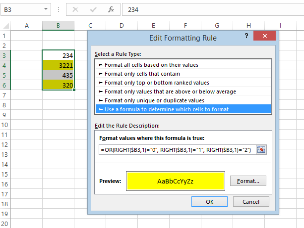
Hope this helps.
Hello Svetlana - Thank you so much for offering your time to all of us...
I want to change the background color of an entire row to the color associated with the results of the conditional formatting of a cell in the row.
Thanks!
Hello Neil,
Just select the entire rows before creating a rule, or you can edit an existing rule and make sure it applies to all the columns you want to highlight.
You can find full details with screenshots and examples here:
https://www.ablebits.com/office-addins-blog/excel-change-row-color-based-on-value/
Hi Svetlana,
What I am trying to achieve is a reporting tool.
I want to have default values and when they change, then have the cell display as red.
So the scenario is A1 = Yes, B1 = No
When the user changes either one, I'd want it to change colour. Is this done through conditional formatting?
Hi Will,
I think you can create 2 rules with the following simple formulas:
For column A: =$A1<>"yes"
For column B: =$B1<>"no"
Hi All,
The numbers "Age" column should be filled in with colors against the status mentioned against each of them.
How can we do this using conditional formatting.
Say for example cell containing "3" should be filled with Orange color.
Age Status
3 Orange
4 Green
10 Red
Hello Dinesh
Here is your solution step by step
let me assume cell A2=3, A3=4 and A4=10
1. Go to cell B2
2. Click on Conditional Formatting
3. Select Manage Rules
4. Click New Rule
5. Select Use a formula to determine which cells to format
6. In the box of "Format values where this formula is true:" type
=A2=3
7. Click on format select fill and select the color you want
8. Click ok again ok and again ok
9. Go to Cell B3 and repeat step 2 to step 5
10. In the box of "Format values where this formula is true:" type =A3=4
11. Repeat step 7 and step 8
12. Go to Cell B4 and repeat step 2 to step 5
13. In the box of "Format values where this formula is true:" type =A4=10
14. Repeat step 7 and step 8
its done.
enjoy.
Hi Svetlana,
i have highlited a column with 3 conditions and i got all the column filled with 3 different colrs as i needed. Now, i need to calculate no. of cells in each color for all 3 colors. can you help me?
please.
thanks.
Hi Varun,
Check out the following VB script to count and some conditionally formatted cells:
https://www.ablebits.com/office-addins-blog/count-sum-by-color-excel/#count-conditional-formatting-color