In this article, you will find two quick ways to change the background color of cells based on value in Excel 2016, 2013 and 2010. Also, you will learn how to use Excel formulas to change the color of blank cells or cells with formula errors.
Everyone knows that changing the background color of a single cell or a range of data in Excel is easy as clicking the Fill color ![]() button . But what if you want to change the background color of all cells with a certain value? Moreover, what if you want the background color to change automatically along with the cell value's changes? Further in this article you will find answers to these questions and learn a couple of useful tips that will help you choose the right method for each particular task.
button . But what if you want to change the background color of all cells with a certain value? Moreover, what if you want the background color to change automatically along with the cell value's changes? Further in this article you will find answers to these questions and learn a couple of useful tips that will help you choose the right method for each particular task.
How to change a cell's color based on value in Excel dynamically
The background color will change dependent on the cell's value.
Task: You have a table or range of data, and you want to change the background color of cells based on cell values. Also, you want the color to change dynamically reflecting the data changes.
Solution: You need to use Excel conditional formatting to highlight the values greater than X, less than Y or between X and Y.
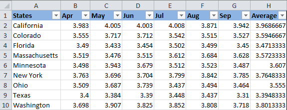
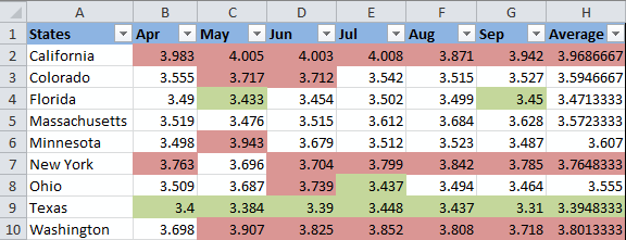
Suppose you have a list of gasoline prices in different states and you want the prices greater than USD 3.7 to be of the color red and equal to or less than USD 3.45 to be of the color green.
Note: The screenshots for this example were captured in Excel 2010, however the buttons, dialogs and settings are the same or nearly the same in Excel 2016 and Excel 2013.
Okay, here is what you do step-by-step:
- Select the table or range where you want to change the background color of cells. In this example, we've selected $B$2:$H$10 (the column names and the first column listing the state names are excluded from the selection).
- Navigate to the Home tab, Styles group, and choose Conditional Formatting > New Rule….

- In the New Formatting Rule dialog box, select "Format only cells that contain" under "Select a Rule Type" box in the upper part of the dialog box.
- In the lower part of the dialog box under "Format Only Cells with section", set the rule conditions. We choose to format only cells with a Cell Value - greater than - 3.7, as you can see in the screenshot below.
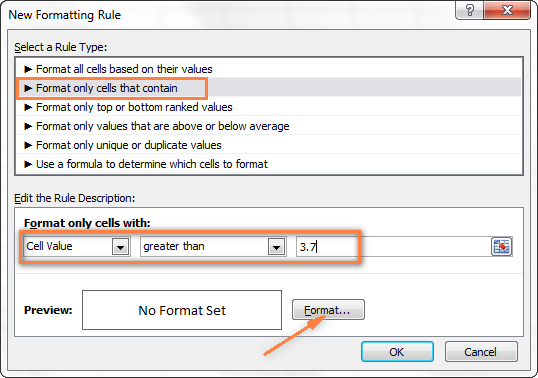
Then click the Format… button to choose what background color to apply when the above condition is met.
- In the Format Cells dialog box, switch to the Fill tab and select the color of your choice, the reddish color in our case, and click OK.
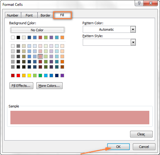
- Now you are back to the New Formatting Rule window and the preview of your format changes is displayed in the Preview box. If everything is Okay, click the OK button.

The result of your formatting will look similar to this:
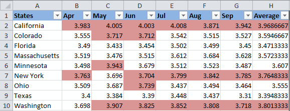
Since we need to apply one more condition, i.e. change the background of cells with values equal to or less than 3.45 to the green color, click the New Rule button again and repeat steps 3 - 6 setting the required condition. Here is the Preview of our second conditional formatting rule:

When you are done, click the OK button. What you have now is a nicely formatted table that lets you see the highest and lowest gas prices across different states at a glance. Lucky they are in Texas :)
Tip: You can use the same method to change the font color based on the cell's value. To do this, simply switch to the Font tab in the Format Cells dialog box that we discussed in step 5 and choose your preferred font color.

How to permanently change a cell's color based on its current value
Once set, the background color will not change no matter how the cell's contents might change in the future.
Task: You want to color a cell based on its current value and wish the background color to remain the same even when the cell value's changes.
Solution: Find all cells with a certain value or values using Excel's Find All function or Select Special Cells add-in, and then change the format of found cells using the Format Cells feature.
This is one of those rare tasks that are not covered in Excel help files, forums and blogs and for which there is no straightforward solution. And this is understandable, because this task is not typical. And still, if you need to change the background color of cells statically i.e. once and forever unless you change it manually again, proceed with the following steps.
Find and select all cells that meet a certain condition
There may be several possible scenarios depending on what kind of values you are looking for.
If you need to color cells with a particular value, e.g. 50, 100 or 3.4, go to the Home tab, Editing group, and click Find Select > Find….

Enter the needed values and click the Find All button.

Tip: Click the Options button in the right-hand part of the Find and Replace dialog to get a number of advanced search options, such as "Match Case" and "Match entire cell content". You can use wildcard characters, such as an asterisk (*) to find any string of characters or a question mark (?) to find any single character.
In our previous example, if we needed to find all gas prices between 3.7 and 3.799, we would specify the following search criteria:

Now select any of the found items in the lower part of the Find and Replace dialog window by clicking on it and then press Ctrl + A to select all found entries. After that click the Close button.

This is how you select all cells with a certain value(s) using the Find All function in Excel.
However, what we actually need is to find all gas prices higher than 3.7 and regrettably Excel's Find and Replace dialog does not allow for such things.
Luckily, there is another tool that can handle such complex conditions. The Select Special Cells add-in lets you find all values in a specified range, e.g. between -1 and 45, get the maximum / minimum value in a column, row or range, find cells by font color, fill color and much more.

You click the Select by Value button on the ribbon and then specify your search criteria on the add-in's pane, in our example we are looking for values greater than 3.7. Click the Select button and in a second you will have a result like this:

If you are interested to try the Select Special Cells add-in, you can download an evaluation version here.
Change the background color of selected cells using "Format Cells" dialog
Now that all cells with a specified value or values are selected (either by using Excel's Find and Replace or Select Special Cells add-in) what is left for you to do is force the background color of selected cells to change when a value changes.
Open the Format Cells dialog by pressing Ctrl + 1 (you can also right click any of selected cells and choose "Format Cells…" from the pop-up menu, or go to Home tab > Cells group > Format > Format Cells…) and make all format changes you want. We will choose to change the background color in orange this time, just for a change :)
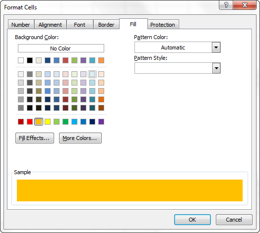
If you want to alter the background color only without any other format changes, then you can simply click the Fill color button and choose the color to your liking.

Here is the result of our format changes in Excel:

Unlike the previous technique with conditional formatting, the background color set in this way will never change again without your notice, no matter how the values change.
Change background color for special cells (blanks, with formula errors)
Like in the previous example, you can change the background color of special cells in two ways, dynamically and statically.
Use Excel formula to change background color of special cells
A cell's color will change automatically based on the cell's value.
This method provides a solution that you will most likely need in 99% of cases, i.e. the background color of cells will change according to the conditions you set.
We are going to use the gas prices table again as an example, but this time a couple of more states are included and some cells are empty. See how you can detect those blank cells and change their background color.
- On the Home tab, in the Styles group, click Conditional Formatting > New Rule… (see step 2 of How to dynamically change a cell color based on value for step-by-step guidance).
- In the "New Formatting Rule" dialog, select the option "Use a formula to determine which cells to format". Then enter one of the following formulas in the "Format values where this formula is true" field:
- =IsBlank()- to change the background color of blank cells.
- =IsError() - to change the background color of cells with formulas that return errors.
Since we are interested in changing the color of empty cells, enter the formula =IsBlank(), then place the cursor between parentheses and click the Collapse Dialog button
 in the right-hand part of the window to select a range of cells, or you can type the range manually, e.g.
 =IsBlank(B2:H12).
- Click the Format… button and choose the needed background color on the Fill tab (for detailed instructions, see step 5 of "How to dynamically change a cell color based on value") and then click OK.
The preview of your conditional formatting rule will look similar to this:

- If you are happy with the color, click the OK button and you'll see the changes immediately applied to your table.

Change the background color of special cells statically
Once changed, the background color will remain the same, regardless of the cell values' changes.
If you want to change the color of blank cells or cells with formula errors permanently, follow this way.
- Select your table or a range and press F5 to open the "Go To" dialog, and then click the "Special…" button.

- In the "Go to Special" dialog box, check the Blanks radio button to select all empty cells.

If you want to highlight cells containing formulas with errors, choose Formulas > Errors. As you can see in the screenshot above, a handful of other options are available to you.
- And finally, change the background of selected cells, or make any other format customizations using the "Format Cells" dialog as described in Changing the background of selected cells.
Just remember that formatting changes made in this way will persist even if your blank cells get filled with data or formula errors are corrected. Of course, it's hard to imagine off the top of the head why someone may want to have it this way, may be just for historical purposes :)
How to get most of Excel and make challenging tasks easy
As an active user of Microsoft Excel, you know that it has plenty of features. Some of them we know and love, others are a complete mystery for an average user and various blogs, including this one, are trying to shed at least some light on them. But! There are a few very common tasks that all of us have to perform daily and Excel simply does not provide any features or tools to automate them or make an inch easier.
For example, if you need to check 2 worksheets for duplicates or merge rows from single or different spreadsheets, it would take a bunch of arcane formulas or macros and still there is no guarantee you would get the accurate results.
That was the reason why a team of our best Excel developers designed and created 70+ add-ins that we call the Ultimate Suite for Excel. These smart tools handle the most grueling, painstaking and error-prone tasks in Excel and ensure quickly, neatly and flawless results. Below is a short list of just some of the tasks the add-ins can help you with:
- Remove duplicates and find unique values
- Merge tables and combine data from different sources
- Combine duplicate rows into one
- Merge cells, rows and columns
- Find and replacing in all data, in all workbooks
- Generate random numbers, passwords and custom lists
- And much, much more.
Just try these add-ins and you will see that your Excel productivity will increase up to 50%, at the very least!
That's all for now. In my next article we will continue to explore this topic further and you will see how you can quickly change the background color of a row based on a cell value. Hope to see you on our blog next week!
 by
by
424 comments
I want that a cell is to automatically get changed its background color when the value is replaced of that particular cell. So that I can get information that this data file has some chamges made by my colleagueue. (like option of Track changes in MS Word)
Hi,
Can't find anything on web to help me out with my problem so maybe you can give a hand on this one:
So, I want to create a drop down list with colors (cells with colors so I can chose the color from a list) but I cannot find how to do it. Then I have another one related to the previous which is I want to do a drop down list based on another one but then have the result color based on the text selected from the drop down menu if that makes sense :D... would be very appreciated if someone can help me with it... cheers
Hello Bruno!
The contents of the drop-down list cannot be colored. The drop-down list uses values, and the color cannot be the value of the cell. However, using conditional formatting, you can paint over a cell after a value is selected from the drop-down list.
Hello! Can I use conditional formatting to highlight all cells in a range that have been changed since X date (date as specified cell A1). As an example, a cell might have $10 one week and be changed to $5 the next week. If this has happened I want to see it highlighted with a red square around it. Note it is a huge table that has an infinite amount of rows and the cells already have other conditional formatting applied. Thanks
Hai,
I just want to highlight the cell if the previous 3 cells in a row contains any numerical value.
Can anyone please help me out.
hello Arjun!
Please try the following formula conditional formatting:
=(ISNUMBER(INDIRECT(ADDRESS(ROW(A1),COLUMN(A1)-3,4))) +ISNUMBER(INDIRECT(ADDRESS(ROW(A1),COLUMN(A1)-2,4))) +ISNUMBER(INDIRECT(ADDRESS(ROW(A1),COLUMN(A1)-1,4))))>0
I hope this will help, otherwise please do not hesitate to contact me anytime.
THANKS
Very Very Thanks
Excellent article. Thanks so much. I found exactly what I needed.
It is really useful. Thank you for this good job.
I looking almost the same but i need to check data value of day of weeks like sunday and saturday and the row from A1 to A8 for example to be colored automatic if they see on A1 Sunday i make calendar for my workstation
1. Select A1:A8
2. Click Conditional Formatting
3. Select New Rule on the pull-down list
4. In a New Formatting Rule window that pops up, select Use formula...
5. In the Edit the Rule Description, Format values... box enter: =(A$1="Sunday")
6. Click Format button
7. Select Fill tab, if you want to change the colour of the background, or Font tab, Color box, to change the colour of the font/foreground
8. Select the colour and OK your way out
If you want to play with the current day of the week, you can modify the formula to: =(WEEKDAY(TODAY(),1)=1)
Thanks
Hi,
I am trying to use the formatting, but no luck so far.
I need to have the whole row to change the colour based on the selection made in one of the columns (status).
Any ideas how this should be set up?
Thanks
Pls., be exact, Aga, so I can give you the exact answer. For as much as you have specified, the answer would be something along these lines:
1. Select the whole row you want to apply the formatting to (by clicking on the row number to the left of the column A)
2. Click Conditional Formatting
3. Select New Rule on the pull-down list
4. In a New Formatting Rule window that pops up, select Use formula...
5. In the Edit the Rule Description, Format values... box enter: =(cell_ref=content), where your cell_ref has to be absolute ($A$1 style) or mixed with fixed column (A$1 style), and content is a numeric or textual value
6. Click Format button
7. Select Fill tab, if you want to change the colour of the background, or Font tab, Color box, to change the colour of the font/foreground
8. Select the colour and OK your way out
1. Select A1:A8
2. Click Conditional Formatting
3. Select New Rule on the pull-down list
4. In a New Formatting Rule window that pops up, select Use formula...
5. In the Edit the Rule Description, Format values... box enter: =(A$1="Sunday")
6. Click Format button
7. Select Fill tab, if you want to change the colour of the background, or Font tab, Color box, to change the colour of the font/foreground
8. Select the colour and OK your way out
If you want to play with the current day of the week, you can modify the formula to: =(WEEKDAY(TODAY(),1)=1)
Sorry, this was the reply for TeamMas7eR
I have a data set that has a distribution very much centered around a static median. If I use the color scale conditional formatting provided I get a data set that is very much yellow with the occasional red and green.
What I need is a conditional formatting where all values above the median have a red color scale and and all values below the median have a green color scale. The values on either side of the median are very much different colors and the intensity of the color is dependent on the value.
Is there an easier way to do this than writing a dozen or more conditional rules?
How would I change cell A3 to reflect what is said in Cell M3?
I'm creating a tracking sheet and I want cell A3 to be blank and only color coded either red or green when cell M3 says Yes(green) No(red). How would I do this?
If your M3 contains textual values "Yes" or "No":
1. Select A3
2. Click Conditional Formatting
3. Select New Rule on the pull-down list
4. In a New Formatting Rule window that pops up, select Use formula...
5. In the Edit the Rule Description, Format values... box enter: =(M3="Yes")
6. Click Format button
7. Select Fill tab
8. In the lowest row of the coloured squares, select the 6th from the left (Green), and click OK
9. Click OK to accept this rule
10. Repeat steps 2. - 9. except:
10.5. In the step 5., the formula is: =(M3="No")
10.8. In the step 8., select the 2nd box from the left (Red)
11. Click Conditional Formatting
12. Select Manage Rules on the pull-down list
13. You should see 2 lines:
Formula: =(M3="No") with an AaBbCcYyZz text on the Red background in the Format column and the =$A$3 in the Applies to column, and
Formula: =(M3="Yes") with an AaBbCcYyZz text on the Green background in the Format column and the =$A$3 in the Applies to column, and
14. Click OK to exit Conditional Formatting Rules Manager
If your M3 contains Boolean values TRUE or FALSE instead of the text, everything remains the same except:
A. Formula =(M3="Yes") changes into a simple =(M3)
B. Formula =(M3="No") changes into a simple =(NOT(M3))
Excellent article. Thanks so much. Found exactly what I needed.
Really helpfull...
I have a problem. I want source of data that contains hours in cells, those cells are coloured filled manually when they they are paid. But what i hope to do is use that data to tell me when how much those hours represent in terms of £. To do this I hope you use another tab pulling in the hours and multiple those hours by various hourly rates. I then have a colour function to tell me how much of these are unpaid for a specific period. But I cant figure out how to pull in the colour of the cell automatically, because it might changed, once they are paid.
How do I apply conditional formatting to a row of names to highlight the cell if the name matches another list of names in another tab
THANK YOU SO MUCH. BEST SITE EVER FOR EXCEL TUTORIAL. TUTORIAL TEACHING LIKE ABC.
Hello,
I need to change the color on the basis the number range.
Ex:- If =4 should go on Red, if in between 3 to 4 should go on Yellow.
Expecting answer asap. Please help me on this:(
Regards
Ghouse
+919916964433
Hi,I have a project management file with main file as project list and a separate worksheet for each project with project details. One of the important information is product order date. I was able to format the date cells to change the color format when the date is less than 30 days away.
But I want to reference that change into the main file so I don't have to review each project tab to see if any of the product deadline is approaching.
For example Project X worksheet has 10 line items with different order date based on when the product will be required. As the date is less than 30 days away the cell for that particular product line changes to Red to alert me. But in order to get that information I have to review each tab periodically. I want if any of the product order date reaches less than 30 day limit I should get an alert (cell format change) in the main file in front of Project X. (Change in any one of a group of cells will alert the user in main file in one cell only)
Please advise if there is a way to do that.
Thanks in advance for your help!
nice
Hi, a little help on formatting that I know should be easy but I can't seem to find.
I'm trying to change the color of a cell based on if it is higher on lower than the cell before it. I need to do that with every cell. If its higher I need the cell to be green and if its lower I need the cell to be red.
Any and all help will be appreciated.
Hi team
I have a row of numbers numbered from 1 to 84 representing 6 years at 12 months per year
Based on the number in a cell in a column before the start of the years I want to be able to GoTo a starting cell under any number from 1 to 84 and fill in a colour starting at that cell reference and continue to Color say x cells based on the value in anthother cell
Thanks very much for your help.
Very appreciative
I really loved it and helped a lot
Here is the formula
TODAY()>DATE(2019,6,19)
I want the contents of the cell to change colour
I know it's true
Conditional formatting does not work....why???
Please help
Excel 2003
Is there anything where even one cell is empty and we want to change whole row bg color. I tried too many times but I failed.
Thank you. What I need to to format a range of cells based on one cell.
IE
If A1 > 0 then color format A1 (the value = 10) and color format A2 (A1 is over 0)
I'm THIS close (' ') to figuring it out.
Thanks
How to change colour of a cell based on the number in the previous cell. Like if I enter number greater than 5 in Column A, in Column B it should be green colour. And if I enter number less than 5 in Column A it should be red colour in Column B.
Very helpful, many thanks :)
Excellent!
Great work! thanks for the help!
Thank you very much.
This was a big help!
I wish to change the color of whole row on the basis of any particular cell's value. How to do this?
They have a lesson that explains how to do just that! :-)
https://www.ablebits.com/office-addins-blog/excel-change-row-color-based-on-value/
Thank you very much for the instruction, it was helpful.
but i still have challenge of changing the background color of an empty cell. will like to get another way of doing that.
Regards
help full thank for sharing
Hi,
I am working on some Demand and Supply data, where you have the Demand value in ,say, cell C3 and Supply value in cell D3. I need to colour background both cells to the same colour for three possible scenarios,i.e. cell C3 is greater than cell D3 then both cells to have a background colour of amber. Also,if cell D3 is greater than cell C3 then both cells to come up red and finally, if both cells equal each other then both cells come up green.
I would then need to format all other cells in the spreadsheet.i.e. cells C3 and D3 represent week 1, the next cells, E3 and F3 would represent week 2 and so on. Each line represents a different entity so would need to format the cells down as well as across.
Sometimes the value of one of the cells can be zero and I need to ensure this also comes up with the same background colour as the cell it i sbeing measured against.
I have tried the conditional formatting but all the cells kept coming up red !
Many thanks for your help.
Kind Regards
Nick
Thank you so much! This was extremely helpful!
thank you for the information
Helpfull
Very helpful and detailed explanation. Really appreciate it
I would like some help please with conditional formatting. We have an inventory sheet that indicates the items and number of items in the store. I have used the Less than function in the conditional formatting to define a change in background colour when and item numbers is reduced below a certain amount. This amount is variable for each item. We have encountered the problem that when new items are added to the inventory and then they are sorted alphabetically, then the conditional formatting stays at the cell position and is not linked to the items number, such that now the formatting applies to a different item with different limits. How can I resolve this? Is there a way to link the conditional formatting to a item rather than a cell? Many thanks in advance for your help
How do you use the best conditional formatting that shows the differences between the amounts in each cell on a column?
budget
237000000
300000000
245000000
250000000
263700000
258000000
260000000
250000000
250000000
250000000
209000000
200000000
225000000
215000000
225000000
225000000
i need to create a formula for conditional formatting. if column D contains "N" then column L should be shaded blue.
how can i do this?
I need this exact same thing. I have a staffing spreadsheet. We are checking everyone's temperature for coronavirus. I have the number of hours someone works in column D and in column E there is an 'X' if they have been checked. I want the E cell to highlight RED if it has no value while the D cell is greater than 0. Anyone know how to do this? Thanks!
Hello Hayes!
If I understand your task correctly, to highlight a cell, use the conditional formatting formula
=IF(AND($E1="",$D1>0),TRUE,FALSE)
I hope this will help
Hi,
Can you help me please!
All I need to do is change the colour (green) of a single cell on a spread sheet if the value of multiple cells in a row are greater than 0. when I try only the first cell in the row changes the single cell colour all the others have no effect.
Kind regards
T
Hi,
How can I condition format rentire row(s) based on the content of one cell/column? E.g. make the entire row green if value in one cell is less than a number?
Thanks for your help.
They have a lesson that explains how to do just that! :-)
https://www.ablebits.com/office-addins-blog/excel-change-row-color-based-on-value/
Hi,
Is there a way to change a blank cell color to red, for example, based upon the value placed in another cell, then turn the red cell to clear once data is placed into the red cell?
Hi there,
So my situation is kind of similar, but different.
I am trying to change the formatting (color) of a number of cells in an array (4 cells in a row) given a value that I am going to input in 1 of those cells. This input will be compared to an array of values already input. So depending on the value of the cell I am inputting, if it is lesser than my base I want it to be compared to, the row will be come green. Or stay white.
This is the rule formula I was thinking about, but can't find better.
=IF($C10+$D10=125, $AF$5 (cell to be compared to), IF($C10+$D10=150, $AG$5, IF($C10+$D10=225, $AF$6, IF($C10+$D10=250, $AG$6, IF($C10+$D10=275, $AH$6, FALSE)))))
And, it does not work. It doesn't adapt dynamically.
Any thoughts?
Thank you.
Hi there - I was wondering if you've found a solution to this issue, as I have recently run into it myself! Its quite frustrating. I'd love if you could share any progress you've made.
its very helpful, thanks a lot !
Hi and thanks for the blog post,
Is that possible to modify the color of a cell regarding the content cell hexadecimal value (without coding) ?
and also modify the cells on the right regarding the different shades of a color (such as https://www.crazy-colors.net/en/hex/1e90ff) ?
thanks!
Hi,
Thank you ma'am. It is very helpful :)
Ma'am,
If I want to apply the colors based on the maximum and minimum values of each row independently for a huge number of rows in a go, what can I do?