The tutorial will teach you how to construct the If match formula in Excel, so it returns logical values, custom text or a value from another cell.
An Excel formula to see if two cells match could be as simple as A1=B1. However, there may be different circumstances when this obvious solution won't work or produce results different from what you expected. In this tutorial, we'll discuss various ways to compare cells in Excel, so you can find an optimal solution for your task.
How to check if two cells match in Excel
There exist many variations of the Excel If match formula. Just review the examples below and choose the one that works best for your scenario.
If two cells equal, return TRUE
The simplest "If one cell equals another then true" Excel formula is this:
For example, to compare cells in columns A and B in each row, you enter this formula in C2, and then copy it down the column:
=A2=B2
As the result, you'll get TRUE if two cells are the same, FALSE otherwise:

Notes:
- This formula returns two Boolean values: if two cells are equal - TRUE; if not equal - FALSE. To only return the TRUE values, use in IF statement as shown in the next example.
- This formula is case-insensitive, so it treats uppercase and lowercase letters as the same characters. If the text case matters, then use this case-sensitive formula.
If two cells match, return value
To return your own value if two cells match, construct an IF statement using this pattern:
For example, to compare A2 and B2 and return "yes" if they contain the same values, "no" otherwise, the formula is:
=IF(A2=B2, "yes", "no")

If you only want to return a value if cells are equal, then supply an empty string ("") for value_if_false.
If match, then yes:
=IF(A2=B2, "yes", "")
If match, then TRUE:
=IF(A2=B2, TRUE, "")

Note. To return the logical value TRUE, don't enclose it in double quotes. Using double quotes will convert the logical value into a regular text string.
If one cell equals another, then return another cell
And here's a variation of the Excel if match formula that solves this specific task: compare the values in two cells and if the data match, then copy a value from another cell.
In the Excel language, it's formulated like this:
For instance, to check the items in columns A and B and return a value from column C if text matches, the formula in D2, copied down, is:
=IF(A2=B2, C2, "")

Case-sensitive formula to see if two cells match
In situation when you are dealing with case-sensitive text values, use the EXACT function to compare the cells exactly, including the letter case:
For example, to compare the items in A2 and B2 and return "yes" if text matches exactly, "no" if any difference is found, you can use this formula:
=IF(EXACT(A2, B2), "Yes", "No")

How to check if multiple cells are equal
As with comparing two cells, checking multiple cells for matches can also be done in a few different ways.
AND formula to see if multiple cells match
To check if multiple values match, you can use the AND function with two or more logical tests:
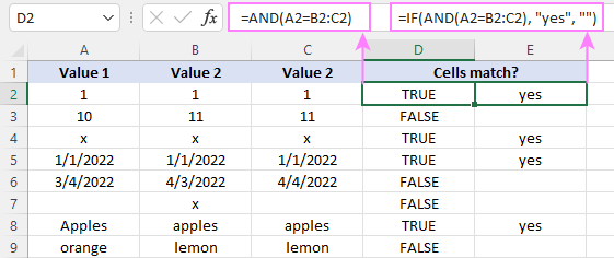
For example, to see if cells A2, B2 and C2 are equal, the formula is:
=AND(A2=B2, A2=C2)
In dynamic array Excel (365 and 2021) you can also use the below syntax. In Excel 2019 and lower, this will only work as a traditional CSE array formula, completed by pressing the Ctrl + Shift + Enter keys together.
=AND(A2=B2:C2)
The result of both AND formulas is the logical values TRUE and FALSE.
To return your own values, wrap AND in the IF function like this:
=IF(AND(A2=B2:C2), "yes", "")
This formula returns "yes" if all three cells are equal, a blank cell otherwise.

COUNTIF formula to check if multiple columns match
Another way to check for multiple matches is using the COUNTIF function in this form:
Where range is a range of cells to be compared against each other, cell is any single cell in the range, and n is the number of cells in the range.
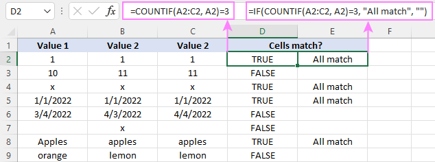
For our sample dataset, the formula can be written in this form:
=COUNTIF(A2:C2, A2)=3
If you are comparing a lot of columns, the COLUMNS function can get the cells' count (n) for you automatically:
=COUNTIF(A2:C2, A2)=COLUMNS(A2:C2)
And the IF function will help you return anything you want as an outcome:
=IF(COUNTIF(A2:C2, A2)=3, "All match", "")

Case-sensitive formula for multiple matches
As with checking two cells, we employ the EXACT function to perform the exact comparison, including the letter case. To handle multiple cells, EXACT is to be nested into the AND function like this:
In Excel 365 and Excel 2021, due to support for dynamic arrays, this works as a normal formula. In Excel 2019 and lower, remember to press Ctrl + Shift + Enter to make it an array formula.
For example, to check if cells A2:C2 contain the same values, a case-sensitive formula is:
=AND(EXACT(A2:C2, A2))
In combination with IF, it takes this shape:
=IF(AND(EXACT(A2:C2, A2)), "Yes", "No")

Check if cell matches any cell in range
To see if a cell matches any cell in a given range, utilize one of the following formulas:
OR function
It's best to be used for checking 2 - 3 cells.
Excel 365 and Excel 2021 understand this syntax as well:
In Excel 2019 and lower, this should be entered as an array formula by pressing the Ctrl + Shift + Enter shortcut.
COUNTIF function
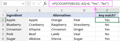
For instance, to check if A2 equals any cell in B2:D2, any of these formulas will do:
=OR(A2=B2, A2=C2, A2=D2)
=OR(A2=B2:D2)
=COUNTIF(B2:D2, A2)>0
If you are using Excel 2019 or lower, remember to press Ctrl + Shift + Enter to get the second OR formula to deliver the correct results.

To return Yes/No or any other values you want, you know what to do - nest one of the above formulas in the logical test of the IF function. For example:
=IF(COUNTIF(B2:D2, A2)>0, "Yes", "No")

For more information, please see Check if value exists in a range.
Check if two ranges are equal
To compare two ranges cell-by-cell and return the logical value TRUE if all the cells in the corresponding positions match, supply the equally sized ranges to the logical test of the AND function:
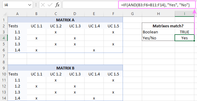
For example, to compare Matrix A in B3:F6 and Matrix B in B11:F14, the formula is:
=AND(B3:F6= B11:F14)
To get Yes/No as the result, use the following IF AND combination:
=IF(AND(B3:F6=B11:F14), "Yes", "No")

That's how to use the If match formula in Excel. I thank you for reading and hope to see you on our blog next week!
 by
by
141 comments
In Sheet1, I have around 150 estate names listed in rows and approximately 106 salary subcategories in columns. I would like to retrieve the results in Sheet2. I have tried using the XLOOKUP function, but I am not receiving the expected results. I have included the formula I used below. Could you please provide assistance in resolving this issue?
=XLOOKUP(B1,Sheet1!$A$2:$A$10,XLOOKUP($A$2,Sheet1!$B$1:$F$1,Sheet1!$B$2:$F$10))
Hello Komala!
Unfortunately, I don't know what results you wanted to get. Also, I don't have the data to check your formula.
I can assume that you tried to search by rows and by columns.
Maybe these articles will be helpful: INDEX MATCH MATCH in Excel for two-dimensional lookup and Two-way (nested) XLOOKUP.
Hi Alexander!
I appreciate your suggestion. I have reviewed the instructions you provided regarding XLOOKUP and INDEX, and I have implemented them in my worksheet. As a result, I am now able to retrieve the data successfully. The formula I utilized is as follows.
=IFERROR(XLOOKUP($A2,SumppgASL2024!$A:$A,XLOOKUP(B$1,SumppgASL2024!$B$1:$DF$1,SumppgASL2024!$B:$DF)),0)
Hello Alexander! your formulas works perfectly!!!
I need your support again.
i need to write couple of IF conditions
A B C D
type quantity Unit Solution
Riba 1 CT
Meso 3 CT
Baklava 5 PAC
Pita 7 CT
Torta 8 PAC
If "Type" is Riba and "Unit" is CT, then multiply by 3
If "Type" is Meso and "Unit" is CT, then multiply by 4
Otherwise everything else should be as it is
Thanks!
Hello Ema!
You can find the answer to your question in this article: Excel Nested IF statements - examples, best practices and alternatives.
Solved :)
Good morning,
I have a scenario where I need to compare two fields to test "true" or "false", which is easy. I only want to compare the fields when both cells have values. If one of the fields is blank then the test should not be performed. I have tried multiple formulas and none work. Can you assist?
Thank you,
Hello Karrie!
Add one more condition to your formula:
NOT(OR(ISBLANK(A1),ISBLANK(B1)))
For more information, please visit: ISBLANK function in Excel to check if cell is blank.
I have this formula
=SUNIF(b2:b5,”a”,d2:d5)
I wish to add a 3rd column a2:a5 “py”
The result is in d15
Hello Paul!
If my understanding is correct, try to use SUMIFS function for two conditions:
=SUMIFS(D2:D5, B2:B5,”a”,A2:A5,“py”)
I want to write a formula as follows:
if cell j9 is equal to or less than c6,
if equal or less than result is c5+2,
if more than J9 the result is c5 +1
My first thought on formula is =if(AND(C6=J9,C6<j9)),(=sum(C5+2)),(=sum(C5+1))
This doesnt work, can you help?
Hello Howard!
You can find the answer to your question in this article: Nested IF in Excel – formula with multiple conditions.
Hi Alex,
Would you please suggest me the formula for the following criteria?
For the following table, product ID in range, in which Product ID 'A01' meet the condition as "Yes" to all the iteration for the Product ID 'A01' in Result received column will return the value "Yes" to All Product result received column for Product ID 'A01' as displayed below:
ProductID, Result received, All Batches result received
A01, Yes, --> No
A02, Yes, --> Yes
A03, Yes, --> Yes
A01, Yes, --> No
A04, Yes, --> Yes
A01, No, --> No
A02, Yes, --> Yes
Thank you,
Mrunal
Hi! Use COUNTIF function to count the number of values that have a specific product ID in column A. Use COUNTIFS to count the number of values under two conditions: the specific product ID in column A and "Yes" in column B.
If the results are equal, use the IF function to return "Yes".
Based on this information, the formula could be as follows:
=IF(COUNTIF($A$2:$A$10,A2) = COUNTIFS($A$2:$A$10,A2,$B$2:$B$10,"yes"),"Yes","No")
Can't thank you enough! Alex. It actually works. Much appreciated your help.
Is there a way to filter this scenario? I have 7 columns and they will each show either YES or be blank.
I want the 8th result column to reflect "COMPLETE" only if all of the boxes are equal and reflect YES. If any of the boxes are blank, or all of the boxes across the row are blank, I do not want the result YES to reflect.
My issue is that when trying to do an all match IF function, they rows that all the boxes are blank also are pulling into the result. I do not want those all blank rows to pull as complete.
Any help would be appreciated! Thanks!
Hi! If I understand your task correctly, the following formula should work for you:
=IF(PRODUCT(--(A2:G2="Yes")),"COMPLETE","")
A mathematical operation turns logical expressions into numbers. If the product of these numbers is 1, this is TRUE for the IF function.
Hello,
I would like to use the following IF formula to confirm if two cells are equal/ balanced, however, it is not working:
=IF(C7=E7,"OK","NOT BALANCED")
C7 and E7 are cells which both contain different formulas, based on other cells, but their results equal the same result, $9.40.
Formula in C7: =B7-A7
Formula in E7: =SUM(F9+F15)
The results returned for both of the formulas in cell C7 and E7 is $9.40 so the IF function should return as "OK" but instead, it returns as "NOT BALANCED".
What am I doing wrong here? Is it possible the IF function is considering the formula in the cells rather than the actual results of $9.40? If that is the case, how can I fix it?
I appreciate any help!
Hi! The value displayed in a cell is not always the actual value returned by the formula. You can see the actual value if you set the cell format to General. In your formula, try using the rounding function. The formula might look like this:
=IF(ROUND(C7,2)=ROUND(E7,2),"OK","NOT BALANCED")
I am finding your tutorials very useful. Thanks.
I have a specific query that I am sure you will be able to solve.
I have a date in say B2
I have a value in say B20
I have a list of all dates in a single column in another sheet (with nothing else)
I want to place the value of B20 in a cell to the right of the date in the seperate sheet that matches B2
Is this easily possible?
Hi! To write a value into a cell based on a condition, you can use the IF function. If I understand your task correctly, the formula might look something like this:
=IF(A1:A10=Sheet1!$B$2,Sheet1!$B$20,"")
Hello.
I'm having a range of numbers and I want to know if there are 2 equal numbers. If there are 2 equal numbers, I want to be written "equal numbers" and if there aren't equal numbers to be written "without equal numbers". But, the range is between same cells except the cell I want to be related to.
As an example, I have the range B2-B11. I managed to get the first cell with the next function =IF(COUNTIF(B3:B11;B2)>0; "equal numbers"; "without equal numbers"), but the next cell is B3 and I can do the formula IF(COUNTIF(B4:B11;B3)>0; "equal numbers"; "without equal numbers") but I want to add the B2 cell there too. How can I add it, without "touching" the B3 cell, and so on?
Hello! Make sure you use an absolute reference to the range of numbers in the formula. Also, since there must be one countable value in the range, replace 0 with 1.
=IF(COUNTIF($B$2:$B$11,B2)>1, "equal numbers", "without equal numbers")
I have two sheets Data and Attendance, with a mix of text and numbers, basically I'm trying to match a student ID, with the type of workshop they attended and if both are true then to return the text cell value in the appropriate row which is Y, N or blank.
The Student ID is in column 1 on both sheets.
I would like to check if Attendance A2 = Data A:A (these are both numbers) and Attendance G1 = Data D:D (these are both text) then I would like to return the text data in Data L:L
Data Sheet
A = Student ID (8 numerical digits)
D = Skill e.g. MH BC
L = Attended Y, N, Blank
Attendance Sheet
A = Student ID (8 numerical digits)
G1 = text MH BC
G2 is cell I want Y, N or to stay blank to appear in.
Hope this makes sense
Hello! Try to use the recommendations described in this article: Excel INDEX MATCH with multiple criteria - formula examples. For example:
=INDEX('Data Sheet'!L1:L10,MATCH(1,('Data Sheet'!A1:A10=A1)*('Data Sheet'!D1:D10=G1),0))
You can also find useful information in this article: Excel XLOOKUP with multiple criteria.
The formula might look like this:
=XLOOKUP(1,('Data Sheet'!A1:A10=A1)*('Data Sheet'!D1:D10=G1),'Data Sheet'!L1:L10)
Want to compare the value of Cell A and B of Sample 1 excel file with Cell A and B of Sample 2 excel file together at a time, if match then the value of cell D (sample 2) will be copied at Sample 1 file.
Please help
Hi! To check two conditions, use the IF AND operator. Read more in this article: IF AND formula in Excel. To learn how to correctly create a reference to a cell in a different workbook, click here: How to create external reference in Excel to refer to another sheet or workbook. Based on your information, the formula might look something like this:
=IF(AND([Book2.xlsx]Sheet1!$A$1=Sheet1!A1,[Book2.xlsx]Sheet1!$B$1=Sheet1!B1,[Book2.xlsx]Sheet1!$D$1,"")
Do you have a formula for this condition : ( if cell1=x and cell2 y → cell3 = z) ? thank you .
Hi! The answer to your question can be found in this article: IF AND formula in Excel.
Hi There, I would love some help. I have two sheets with the same data range, State and Email. I am attempting to cross reference if the two sheets have matching information. I have used this formula but it is not working.
=IF(AND(C2='Response Data'!B2,'Agent TMT State Data'!,D2='Response Data'!C2),TRUE
Hi! Since your formula is not completely written down, and I do not have your data, I cannot verify it. 'Agent TMT State Data'!,D2 - mistake, no comma needed. C2 - there is no reference to the worksheet. Use the recommendations I gave earlier: Compare two columns for matches and differences. Or give an example of what you want to compare.
Hi Alex,
I have two worksheets named Response Data and Agent TMT Data. Each worksheet has a column for State and Email, there are roughly 6000 records.
I want to create a formula that will give me a response of Match/No Match or True/False if the row that contains the data for state and email is not matching.
EG: Response data has C2 test@test. com and D2 Texas, TMT Agent data has the same information in the worksheet (test @test. com and Texas in the same row)
I hope this makes sense
Hello! If I understand your task correctly, the following formula should work for you:
=ISNUMBER(MATCH('Agent Response Data'!C2&'Agent Response Data'!D2, 'TMT State Data'!C2:C30&'TMT State Data'!D2:D30,0))
We have a tool that can solve your task in a couple of clicks - Compare Two Tables. This tool can compare two tables or lists by any number of columns, identifying matches/differences (like formulas) and highlighting them (like conditional formatting). The tool is included in the Ultimate Suite for Excel and can be used in a free trial to see how it works.
Hi, I have a big excel sheet containing data on M&As which I have to combine.
I have three columns which have to match, two columns with Ticker Symbols and one with the corresponding ISIN code of a company. If the ticker symbols match I want to get the corresponding ISIN code for the company and its deal (in some cases it is one deal, others could be 20). But for some reason it does not check all cells, rather if I write a function it automatically jumps to the next ticker symbol. Do you perhaps know what function to use?
Hi! I can't guess which formula you're using. But if you're searching using VLOOKUP or INDEX MATCH, remember that these will only find the first match. If you want to get all the values from the third column where the values from the first and second columns match, use the FILTER function and these instructions: Excel FILTER function - dynamic filtering with formulas.
Unfortunately, the information you have provided is not sufficient for us to recommend a formula to you.
Can I get help with this formula? I'm getting a syntax error message when I enter this and can't figure out the issue. I just want it to pull a value based on different ranges.
=IFS(COUNTIF(Reference!B2:B64,B3)>0,Reference!B1, [COUNTIF(Reference!C2:C64,B3)>0],Reference!C1, [COUNTIF(Reference!D2:D64,B3)>0],Reference!D1)
Hi! Do not use [ ]. Try to follow the recommendations from this article: Excel reference to another sheet or workbook (external reference). I hope it’ll be helpful.
I have two drop down list B2 and D2. If B2 equals to a text then D2 should only have a certain lot of values/text available to use and the rest must be grey out. what formula to i use?
Hi! To make the values in the second drop-down list depend on the first drop-down list, use these instructions: How to make a dependent (cascading) drop-down list in Excel.
Hi,
I have two different diagrams. What they have in common is that they both have one column with the same material number, but sorted in different rows.
But, the first diagram have a column with the change of the quantities of how much materials will increase or decrease.
And the other diagram have a cost per unit column.
I must somehow figure out how much will the cost increase or decrease in every row for every material number.
Maybe I can use the material number. If they match equally,then I can multiply the Change in Quantities with Cost per Unit. But how?
Hi! With the VLOOUP function, you can get the price for each material number from the second table. Look for the example formulas here: Excel VLOOKUP function tutorial with formula examples. For each material, you can then calculate the increase or decrease in cost using this table.
I want to get a yes or no answer. If G3 equals H1 or I1 then no, otherwise yes
Column G could have PP01, PP02, PP01A, PP02A. H1 = PP01, I1 = PP02
Hi! Try to use the recommendations described in this article: Excel IF OR function with formula examples.
For example:
=IF(OR(H1=G3,I1=G3),"no","yes")
First off, great simple instructions! Very helpful.
Using this formula =A2=B2 (If two cells equal, return TRUE), is there a way to have True in Green color font, and False in Red color font.
Hi! Font color definition in Excel is not a matter of standard functions. Instead, VBA and user-defined functions are needed. An example of such functions is provided in this guide: How to sum and count cells by color in Excel.
Here is an example formula to compare font color in cells:
=GetFontColor(A2)=GetFontColor(B2)