The tutorial demonstrates a number of techniques to compare and match two or more columns in Excel with formulas, conditional formatting and the specialized wizard. Continue reading
Comments on: How to compare two columns in Excel for matches and differences
 by Svetlana Cheusheva, updated on
Comments page 3. Total comments: 271
Hello,
I have 2 excel with more than 500 row in both excel (peoples name)
Since full names of peoples are not exactly same in both excel but for some name first name is matching and for some name, middle and last name is matching.
so what formula can we use to find matching word between these 2 excel.
thanks.
Hello Shiv!
Please describe your problem in more detail. Write an example of the source data and the result you want to get. It’ll help me understand it better and find a solution for you. Thank you.
did you get a reply
Hi,
I have 2 columns: Column C - having all my dates when my customers require delivery and Column E – having all my dates when I will be finished. I want my dates in Column E to be GREEN if it is less than Column C and RED if it is greater than Column C. Can you assist with a formula or show me how, I’ve tried through conditional formatting and struggling, please assist.
Hello Cherry-Lee!
You need to use conditional formatting. I recommend to study this article on our blog.
Hello there,
I have 30 questions (from Row 2 to 31 and Row 1 is header row). Column A is for question number, Column B is for correct answer, Column C is student 1 answer, Column D is student 2 answer and so on..
I just want total correct answers for each student in row 32. I dont know if we can do anything with countif or sumif.. but what i did was, I added 1 column in the right for each student and then i put a simple formula if his/her answer matches with column B then 1 else 0, and the summing up in row 32.. is there any way to avoid those extra columns?
Hello!
Use formula =SUM(--(B2:B31=C2:C31))
Never mind.. i got my answer.. using sumproduct..
Hi there,
I need help, bellow here is the scenario.
Column A = Client names
Column B = Manager name
Column C = Sign off date
Identify any records where “Client Name” paired with “Manager name” has answer to “Sign off date” with dates that are not equal.
Hello!
I propose to select the necessary entries using conditional formatting. Read about it on our blog here.
I have an interesting problem. I am developing a project with 7 teams of 15 people on each team. One person may not be on more than one team. I want to find if I have put the same person on more than one team and highlight the name in both cells. I think it is a look for duplicates, but I cannot find a solution across 7 non-contiguous columns. Thank you so much for your help.
Hello Keith!
You can learn more about highlight duplicates in Excel in this article on our blog
Hope you’ll find this information helpful.
NEED HELP.
SCENARIO:
CELL A1= 3/6/2020
CELL B2= EMPTY
CELL C3=+10 DAYS IF A1 HAS DATE, +10DAYS IF B2 HAS DATE AND A1 IS EMPTY, IF BOTH BLANKS IT RETURNS TO ZERO VALUE.
WHAT IS THE FORMULA THIS SCENARIO?
Hello Fred!
If I understand your task correctly, the following formula should work for you:
=IF(A1>0, 10,IF(B2>0, 10,0))
Thank you so much, as usual, you answered question with multiple varying excel features in a well explained, organized, and documented fashion. The only downside is that you've spoiled me, and I get frustrated with other websites that are not of this caliber.
Thank you, Mike! We'll do our best to keep the bar high :)
Hi,
Below is the data,
Sale order have a some of line items and result is three type A, B, C
For one sale order all line item has C means , result should come as Completed
Sale Order # Line # Status
10045 10 A
10048 20 C
10045 30 C
10045 40 C
10045 50 B
10045 60 C
10046 10 C
10046 20 C
10046 30 C
10046 40 C
10046 50 C
10046 60 C
=IF((P2=L:L),IF(N:N="C","Completed","Not Completed"))
Pls confirm
Saran:
If I understand your question this should work:
=IF(C2="C"',"Completed","Not Completed")
Then just copy the formula down the column to get the results for the respective data. No need to enter a range as in "L:L".
Thanks so much for this tutorial. I've read each response but still haven't found the solution I need. How can I perform a case insensitive partial match from one column to the next? Example.
Column A
green
red
brown
Column B
The green tree
Orange Leaves
Brown Dirt
I would like to search all the phrases in Column B with the words in Column A.
Desired Outcome:
The Phrase "The green tree" in column B should be identified because the word "green" from column A was found.
The Phrase "Brown Dirt" in column B should be identified because the word "brown" from column A was found.
I've scoured the web looking for a solution and I haven't found one that can be easily used without the knowledge of writing code.
Have you been able to find a solution for this? I have the exact same issue. I only need to find a partial match and then sum it all up. I have over 80k (x3) line items to search...
Example four does not do what you say. It does not compare two columns. It compares all cells in the columns; therefore, it will highlight all duplicates even if they are in the same column.
Hi Doug,
You are absolutely right. Don't know what I was thinking. I have removed that example from the article. Thank you for pointing that out!
Hello. I have a problem. I have been given a spreadsheet of students expected and actual grades in different subjects.
I need to format the data so that if the expected grade is higher than the actual grade both turn red. if the actual grade is higher than the expected grade they both turn green and if both grades are the same they turn yellow.
never mind. I found a solution that works
I have a list of items and all have distinct names. I need to compare the items with a list of known partial matches and have the result be the partial match. For example:
Distinct list:
F-daniel-01
R-rose-20
C-daniel-03
T-bob-35
A-kevin-36
Partial match list:
daniel
rose
bob
kevin
Result:
F-daniel-01 | daniel
R-rose-20 | rose
C-daniel-03 | daniel
T-bob-35 | bob
A-kevin-36 | kevin
Any advise would be great
I have the exact same problem and so far I have not been able to find a solution.
How to verify if the names in col A have a match in col B using one, or two words contains or any idea how can be done. Thank you
COLUMN A COLUMN B
ANGEL MARIE DIZON ANGEL MARIE E DIZON
OSCAR LUCAS MARK LUCAS MARK OSCAR
JULIE LIM MAN AREVALO
REYNOLD B WILLIAMS JULIE ANN LIM
JEN MARIE YU REYNOLD WILLIAMS
MAN AREVALO B JEN YU
STARK JOHNSON ARCH MAY TAN
ARCH TAN JOHNSON STARK
Jejemole:
I think the only way Excel can be used to help you with this is to use the Fuzzy Logic add-in from Microsoft.
If you Google MS Fuzzy Logic you'll see the address. The description and instructions are there, too.
when excel worksheets have been programmed using these conditions, can we found back the corresponding vba code associated?
J-Law:
In the Developers Tab there is a tool to View Code. When you select it the modules are available. There you can select the module and you'll see the code.
If you don't have the Developers tab active, in 2016 you can see how to open it and how to use the tools in Excel by entering: "Display the relationships between formulas and cells" in the Tell me what you want to do box and click the help option.
Then you'll see the article which addresses your question.
I am a beginner in VBA. i need to compare the values in co11 of row1, row2, row3 so on till the end of the file. if r1c1 = r2c1 then i want to add the values in r1f1 and r2f1, if not equals go to next row. if the value in b1 of row1, row2 and row3 are equal then i wish to add the value of col f in all the rows.
please guide me Ms svet
Prasad:
Assisting users with VBA questions is beyond the scope of this blog. There are many other sites that can help you. Google "Beginner VBA Help" and you will find them.
Hello I have a situation where i have column A with part number and column B which captures status if "quote recd" or "no quote".
the quotes are valid for 7 days. if i receive the same part number request on the 10th day i want to highlight that part number to check the status column and highlight if we have ever received quote for that part number.
i want to use conditional formatting to highlight that part number if anywhere in Column B it finds "quote recd".
Abbas:
Where are the dates stored? Wherever they are you can follow the same procedure to highlight them as outlined below.
If you want to highlight the B cell if it contains "Quote Recd" then select the cells that you want to highlight, go to Conditional Formatting, select the "Cells Equal To:", type Quote Recd" in the field and choose the formatting color of your choice. Click Save and then OK. Your cells should be filled with the formatting of your choice.
Hello!
I have 2 different sheets. On sheet2, I want to find the PN 4324568 at what is the location and it pulls the data from sheet1 which is location 14. What formula do I need?
Sheet1
Col A
Row 1 PN 4324568
Row 2 Location 14
Sheet2
Col A
Row 1 PN 4324568
Row 2 Location ??
Thanks, Dan
Dan:
If you structure your data in sheet 1 by having PN in column A and their Location in column B you can do a VLOOKUP on sheet 2 like this:
In Sheet 2 column A enter the Part Numbers. In column B
directly across from the first part number enter
=VLOOKUP(A2,Sheet1!$A$2:$B$25,2,False) where A2 is the first part number for which you need a location and also
where Sheet1 A2:B25 are the cells which contain all of the part numbers and their locations.
I asked something similar in the countif section,but this may be a better place to ask. I'm looking just to get the number of matches between two columns when compared row by row. Is there any way to do this.
If I understand your question, this is how to get the sum of matches in two ranges of data:
=SUMPRODUCT(--(A39:A45=B39:B45))
Where A39:A45 is the first range of data and where B39:B45 is the second range of data.
So, this answers the question "What is the sum of the number of matches in these two ranges?" or put another way, "How many matches are there in this data?".
New _Position code
JOB049130401803012001-002
JOB052110609801019002-004
JOB055350101805042003-005
JOB055350101805042003-006
JOB055350101805042003-007
JOB073850101805042003-004
JOB073850101805042003-005
JOB077910609801019002-003
JOB077912002801019002-001
JOB077912002801019002-0010
JOB077912002801019002-002
JOB077912002801019002-003
JOB077912002801019002-004
JOB077912002801019002-005
JOB077912002801019002-006
JOB077912002801019002-007
JOB077912002801019002-008
JOB077912002801019002-009
JOB078310107801019001-005
JOB080650101805222015-005
JOB086112001801039001-005
JOB086112001801039001-009
JOB086112001801039008-006
JOB086112001801039016-005
JOB086112001801039017-006
JOB086112001801039025-005
JOB086112001801039025-006
JOB090612002801152011-001
JOB090612002801152011-002
JOB090612002801152011-003
This is my list where i need to know which no is free to put in the end like -004,-005 etc which i have to put to create unique code. kinldy help me
JOB077912002801019002
Hello,
I'm afraid there's no easy way to solve your task with a formula. Using a VBA macro would be the best option here.
However, since we do not cover the programming area (VBA-related questions), I can advice you to try and look for the solution in VBA sections on mrexcel.com or excelforum.com.
Sorry I can't assist you better.
May I ask how to pull out the text/string data different from column A (ie A2:A10) and Column B (B2:B10) to cloumn C
An example of raw data set:
A B C
Student Name: Student Name: Missing:
Tom Tom Jerry
Jerry Catherine Sam
Catherine Ada
Ada
Sam
Thank you!
Hello,
Please try the following formula:
=IFERROR(INDEX($A$2:$B$10,SMALL(IF(($B$2<>$A$2:$A$10)*($B$3<>$A$2:$A$10)*($B$4<>$A$2:$A$10)*($B$5<>$A$2:$A$10)*($B$6<>$A$2:$A$10)*($B$7<>$A$2:$A$10)*($B$8<>$A$2:$A$10)*($B$9<>$A$2:$A$10)*($B$10<>$A$2:$A$10),ROW($A$2:$A$10)-1),ROW(A1)),1),"")
Please note that this is an array formula. You should enter this formula into the first cell in column C, hit Ctrl + Shift + Enter to complete it and copy the formula down along the column. Just select the cell where you've entered the formula and drag the fill handle (a small square at the lower right-hand corner of the selected cell) down.
Hope it will help you.
How to compare 2 columns to find the match exist or not. I need the formula which compares B1 with A:A. If Match found 1 else 0. I tried =IF(B:B=AA, 1,0) didn't work.
A B
0001165186 0094713197
0001166595 0097094894
0001166619 0094640211
0001190181 0097058341
0001196342 0016685760
0001213475 0016748842
0001216979 0016760276
0001217648 0097012553
0001222292 0097075931
Hello, Sarah,
Please try this formula:
=IF(ISNA(VLOOKUP(B1,$A:$A,1,FALSE)),0,1)
Hello,
For work I am tasked with downloading customer Forecasts and updating our backlog accordingly. it is a very time consuming process. there are multiple parts that are on multiple different purchase orders with quantities and dates varying on a monthly basis. the changes are not that frequent but I have hundreds of rows to go through. I am looking for a way to quickly find changes that have occurred month to month however I need to hold reference to the part number, purchase order, quantity and date. have you any thoughts on how I may be able to do this?
Hello, William,
if I understand your task correctly, we have the add-in that may help you.
Please take a look at the Compare Two Tables tool from the Duplicate Remover add-in. With its help you'll be able to find unique records or remove duplicate values between 2 worksheets.
You can download a fully functional trial version to test the add-in and see if it work for you from this web-page:
https://www.ablebits.com/downloads/index.php
Hope this'll help!
Hi
I want to compare Data in 2 columns A and B and want to highlight the different words only. Eg . my A1 CELL contain Apple, Sweets, good
B1 cell contains
Apple, sweets, pizza, car
In above two cells in A1 good is extra word which is not present in CELL B1. Where as Cell B1 contains words " Pizza, car "which are not present in excel so how to highlight only these different words
I have lot of Data
Hi, Sandy,
I’m afraid there’s no way to highlight only duplicate words in Excel. All the formulas and our add-ins will select or highlight the entire cell.
I can only advise you to ask around Mr.Excel forum in case they come up with some VBA code for you.
I wish I could assist you better.
Salaam everyone.
I have two excel columns each containing 63,000 values. I want to find out all the values where entries of column A are greater than those of column B. How can I do that?
Thanks in advance
Stay blessed.
Hello Fiaz,
You can enter the following formula in the first cell with data, say A1:
=IF(A1>B1, TRUE, "")
Then, copy the formula to the entire column. And after that sort or filter your dataset by the formula column.
I need a formula that will help me identify duplicate parts/product at different pricing. When I use the conditional formatting on both columns all of the cells are highlighted because it's looking at just the columns as duplicates.
Hi, Eva,
I managed to do that in the following way:
1) I decided to use a helper column (C) that checks if the product (A1) is duplicated and its price (B1) is unique with the following formula:
=COUNTIFS(A:A,$A2,B:B,"<>"&B2)
If the condition is true the formula returns 0, since it can't find any duplicated products with unique prices. Otherwise, it returns 1.
2) I created a following conditional formatting rule:
=$C1>=1
and applied it to my table =$A:$C
As a result, I can see all the duplicate products with unique prices highlighted in yellow.
Try to do the same with your data, hope it helps!
Hi Meli,
As i can see it's time sheet of employee. I understand your query. But without sample sheet i am unable to put formula here. so share any short sample sheet fot add formula.
In Time Out Time In Time Out Time
11:00:00 AM 8:30:00 PM 10:50:00 AM 8:40:00 PM = PRESENT
11:00:00 AM 8:30:00 PM - - = Single Punch (This should be absent) Absent
11:00:00 AM 8:30:00 PM 11:30:00 AM 8:35:00 PM = LATE
11:00:00 AM 8:30:00 PM 11:00:00 AM 7:00:00 PM = EARLY
11:00:00 AM 8:30:00 PM 11:30:00 AM 5:35:00 PM = LATE/EARLY
11:00:00 AM 8:30:00 PM 8:45:00 PM - = Single Punch Absent (This should be SP)
11:00:00 AM 8:30:00 PM - - = Single Punch Absent
Not understand the question dear.
Scenario1 :
Check text "abc.AD" in sheet one, and return the next two cell values in sheet two.
Note: The unique text is not in same column.
Sheet 1 :
Col10 Col11 Col13 Col14 col15 abc.AD Test NOP
abc.AD Ext NOP
abc.AD Int NOP
Let me know if this helps
Need help,
I'd like to be able to compare two cells with unique strings
Ex. A1 = xyz0_ok_hmu1-ty
B1 = ok1_ty
I want it to be able to recognize that it is similar to a minimum of 2 ordered letter matches and be highlighted as "similar". If it is able to ignore multiple delimiters, that would be cool too.
Hello, Earl,
I'm afraid that existing Excel functions won't help since the comparisons are too vague, if I may say so. We can only advise you to try and use Fuzzy Lookup Add-In for Excel from Microsoft.
btw, the strings are a bunch of acronyms that doesn't make sense, and people have their own way of writing it therefore there are a lot of differences and minimal similarities.
I need help writing a formula to find matches between a column in SHEET1 and a column in SHEET2. Goal is to get "Match" inserted into Column B, SHEET1 if there is a match between Column A and Column B.
I tried:
=IF(A2=$SHEET2$,B2,"Match","") but this didn't work. Can someone help me out please!
Data:
Column A, SHEET1
12AB1250
12AB1251
12AB1252
Column A, SHEET2
12AB1250
12AB1251
12AB1252
12AB1253
12AB1254
12AB1255
Thanks in advance!
=IF(A2=A3,"Match","No match"
Copy and paste above formula and A1 delete and select Column A, SHEET1 and A3 delete and select Column A, SHEET2 . it will work
Hi ,
How to compare two cells whether another cell contains same word,
Location Code Description Location from part no Status
LEAF SPRING FRONT REAR AXLE PARABOLIC SPRING FALSE
Thanks
Hello E Sivakumar,
Please, you can use the following formula:
=IF(A1=B1,"match", "no match")
Hello,
I have two data sets (sheets), first columns in both the sheets have data that can be matched. Based on the first columns, I want to create a new data set having the expanded data for each of the columns.
Thanks.
Hello Rishikesh Shetty,
Please try Merge Tables Wizard to see if it can help with your task.
Please use the link below to download and get additional details:
https://www.ablebits.com/excel-lookup-tables/index.php
I have 2 sheets. 1 has a column with 14 digit numbers representing products. The 2nd sheet has a column with 10 digit numbers also representing products. Product descriptions are different in each sheet. I want to verify the list of 10 digit numbers are included within the sheet with 14 digit numbers. Can you help? Thanks!
Hello Jen,
For us to be able to assist you better, please send us a small sample table with your data in Excel and include the expected result. Thank you.
I need a formula to count how many times column A has a ON and NS that represents a CU in column B. In the case below ON and NS represent a total of 3 CU's in column B
A B
ON CU
BC CU
AB CU
ON CU
NS CU
NS BA
Eg. =+COUNTIFS(QtradePartners!B3:B136,"=ON",QtradePartners!B3:B136,"=NS",QtradePartners!C3:C136,"=CU") ... THIS IS NOT WORKING and I think it makes sense that it doens't work... Anyone help?
Hello Marc,
Please, you can use the following formula:
=COUNTIFS(A:A,"ON",B:B,"CU") + COUNTIFS(A:A,"NS",B:B,"CU")
List 1 List 2
1 a
2 a
3 b
3 b
1 a
3 c
1 d
Hello, please help me in the above example. I want to check if list 1 and List 2 has same row values. Like first row is same as the fifth so row 3 and 4.
WHat formula should I use.
Hello Ashok,
Please, you can use the following formula:
=IF(COUNTIFS(A:A,A2,B:B,B2)< 2,"no match","match")
Hello
I have two excel sheets
One sheets boys sheet mention name, gotra, year, qualification salary
second sheets girls mention name, gotra, year, qualification salary
how we can match it
Hello Chandan,
Please try Duplicate Remover Wizard to see if it can help with your task.
Please use the link below to download and get additional details:
https://www.ablebits.com/excel-suite/find-remove-duplicates.php
Hi, whuch formula should I use if I want to compare 2 excel sheets. 1 has been revised and 1 has no changed.
please help!!!! Thank you
Hello Michelle,
Please check out the below tutorial, you will find a few solutions there:
How to compare two Excel files for differences
i love you.
I fully comprehend, by virtue of your tutorial, as to how to compare two excel files for differences. But then I need learn how to compare the two excel files (and also the two/more columns/rows within an excel file) for matches or similar entries.
Thanking you in anticipation.
Thanx for such an informative article over excel,still struggling to find the solution ,Pl help if possible.
I've two columns in which one column say B having exhaustive values,while in another say column A ,some values are missing.How to ascertain either through Vlookup,Countif or If,which values are missing. Here,it is to be noted that all data in A is in column B,but vice versa is not true. Just wanted to know missing data. Pl help in getting formula for the same.Total entries in column A is less than column B(vertically) Plzz..
Hello Avinash,
If my understanding of the task is correct, you need to identify the values that are present in column B, but not in column A. If so, you can use the following formula:
=IF(COUNTIF($A:$A, $B2)=0, "missing", "")
Where B2 is the topmost cell with data, ignoring column headers.
When you copy the formula down the column, the word "missing" will appear in the rows containing data in column B that do not appear anywhere in column A. To get a list of missing values, apply Excel's auto-filter, filter the formula column by "missing" and copy the filtered values in column B.
if column A has names and column D has dates. Is there a way to highlight equal dates that belong to the same name?
Hello Jonathon,
You can create a conditional formatting rule with the following formula:
=COUNTIFS(A:A, A1, D:D, D1)>1
kindly help me to assign the remarks of attendence as excellent, good or bad based on the student attendence. It will be mentioned in range as 95-99 as Excellent,90-94 as good, 85-89 as average and like.
kindly reply
Hi Manoj,
You need nested IF functions for this. For example:
=IF(A2>=95, "Excellent", IF(A2>=90, "Good", IF(A2>=85, "Average", "Poor ")))
Hello,
I am struggling with how to compare values, and if there is a match, insert a new column. For example, sheet 1 has:
Column A has server names, and will contain duplicates (column B contains application name, multiple app's can run on the same server)
Another spreadsheet (sheet 2) has unique server names by Datacenter (1 Excel sheet for each datacenter). I planned on copy/paste it into column D on sheet 1. If there is a match between column A and D, add a value (the value would be the same each time, as I am pasting only datacenter 1, then datacenter2, etc.) for the Datacenter into column C.
Hope that made sense, and thank you in advance!
I think I found a useable way to get this done, but not ideal. I'll compare the values, if it matches, write MATCH in column C. Then just replace the word MATCH with the Datacenter I am running it for. After a few runs, I'll be done, since I will paste one DC at a time. :-)
Hi I want to compare just first 10 digits of the two cells.What formula can I use.
Did you find an answer for this Deeba? I need it too
Please help me! I have 2 column a and b. "A" column have frutis information. "B" column have rates. The problem is a and b both have duplicate values. A have multiple time "orange". "B" have different rates sometime same rate. I have to find out does the orange has same rate all the time or different rate. If same rate than it has to display match if different rate. Than mismatch
Hello Gokul,
You can use our Duplicate Remover add-in:
https://www.ablebits.com/excel-suite/find-remove-duplicates.php
- Select your table and click on the Dedupe Table icon;
- Select columns A and B to compare rows of values;
- Choose the option to "Add the Status column"
The add-in will mark those rows that have the same fruit names with the same rates.
I need a mark to find duplicates in an excel sheet.
The problem with the records are, they are not exactly the same.
There is always one or more field(s) that differs from each other.
I want to have an automatic way of recognizing this cases.
Hello,
It sounds like our Fuzzy Duplicate Finder add-in will help you:
https://www.ablebits.com/excel-find-similar/index.php
It lets you specify the number of different characters and make the found values identical if necessary.
Hi all,
I would appreciate your help with the following:
I would like to compare two columns, let us say Column A and Column B, looking for duplicates. If a value in Column A has a match value in Column B, I would like to format the cells of the same duplicate value with the color (the colors are random and different for each match). This is if A12 = B30, the color will be red. And if A20 = B1, the color is green and so on.
Regards,
Ali
Hello Ali,
I'm sorry, but there is no simple way to do this. You can have a custom tool developed for you, but as soon as there are over ten values that have duplicates, you can only use the color shades that may be difficult to differentiate.
It may be better to create a conditional formatting rule to check duplicates of a particular value in column A and in column B, then change the rule to see the duplicates of the next value, and so on.
Hi, I need help with a formula. In my example, I am comparing dates between 2 columns (production dates), and I highlight only rows where the dates do not match. I wish to add to the existing formula, so that the comparison (and highlight) is not made if a third column is >1 (which would mean the order has already been produced). My intent is to focus on as-yet unproduced orders, and eliminate the highlight on orders already in stock.
Thank you!
Hi Joseph,
You can create a conditional formatting rule, choose to "Use a formula to determine which cells to format" and enter the following formula:
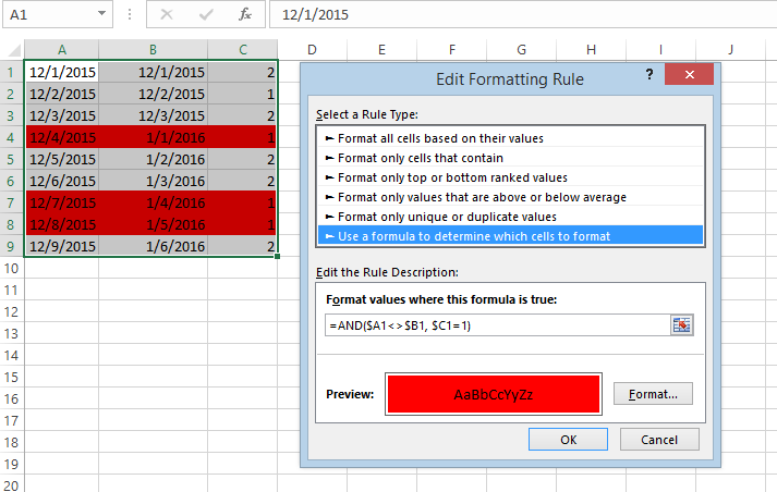
=AND($A1<>$B1, $C1=1)
Here columns A and B contain dates, and column C is the one to check for value "1":
Hi there, the article is very helpful, however I struggle with comparison where some empty cells are included.
Your "Compare multiple columns for matches in the same row" Example 1 is what I was searching for, but it doesn't work if there are empty cells in between.
Say A1= MARK, B1= MARK and C1 is empty, the function gives an error. How can I ignore those empty cells and still the answer to be "match".
Thanks!
Hello Yulia,
If blanks occur only in one of three values in the same row, please use the following formula:
=IF(AND(IF(AND(NOT(ISBLANK(A1)),NOT(ISBLANK(B1))), A1=B1, TRUE), IF(AND(NOT(ISBLANK(A1)),NOT(ISBLANK(C1))), A1=C1, TRUE), IF(AND(NOT(ISBLANK(C1)),NOT(ISBLANK(B1))), C1=B1, TRUE)), "Full match", "")
If you may have blanks in two of three values in the same row, please use this formula instead:
=IF(COUNTBLANK(A1:C1) > 1, "",IF(AND(IF(AND(NOT(ISBLANK(A1)),NOT(ISBLANK(B1))), A1=B1, TRUE), IF(AND(NOT(ISBLANK(A1)),NOT(ISBLANK(C1))), A1=C1, TRUE), IF(AND(NOT(ISBLANK(C1)),NOT(ISBLANK(B1))), C1=B1, TRUE)), "Full match", ""))
Hi Irina,
actually I have found another option: =IF(AND(OR(A1=B1;B1="");OR(A1=C1;C1=""));"ok";"error")
A little bit primitive, but for the purpose works good
Thanks
Yulia
how to check column 1 caste oc; column 2 male or female
how to count caste oc how many female and how many male ?
Hello Ram,
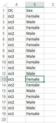
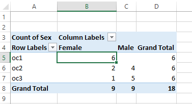
It sounds like you need to add a Pivot Table. We assume your data look the following way:
- Select your data, go to Insert tab in Excel and click on Pivot Table
- Drag column 1 to Rows
- Drag column 2 to Columns and to Values
You will get a count for each oc the following way:
I am wondering if possible to take column A make a match to the bestest (does not have to be 100% exact) match in column B and to say be able to copy that information back to where I want it to be. Doing some url links from data feed and testing idea's like this and hoping to come up with a better answer than doing it by hand. I got 519 rows in column A (menu name for links for website, etc) and 7546 rows in column B from data feed with the end to the links I want to make. Column A is say Women's Active Clothing Or Womens Active and Column B (has in the 7546 rows) a match like clothing & accessories > women > active (this is exact of how they look). I want to match them up then make a url out of it later like mysite.com/products/category/clothing & accessories > women > active to assign to menus like Women's Active Clothing. If any one has an idea please let me know. Am test trialing the software but yet not figured out or if possible to do some thing this hard
Hello, Rod,
For us to be able to assist you better, please send us a small sample table with your data in Excel and include the expected result. Thank you.
Need some help please. I have 3 separate cells, each ca contain variable data
e.g. Cells A1 and A2 can contain one of the following P, p, pi, pe,F, f, -, untested, Cell A3 can contain P,p,F,f,-,untested - what I want as a result in A4 is - If A1 and A2 and A3 all contain P or p(i or e also)then ALL OK, IF A1 or A2 or both contain an F or f but A3 = P or p then A4 should read T OK but prob. If Ai and A2 have P,p,pi,pe but A3 is F then A4 should read T OK up to x-point. If A1,A2 and A3 all contain an F or f then A4 should read T F
Hope you can help - Many Thanks
I've a problem in counting the number of appearing of the data in 2 adjcent cells in a same row.
Say the row is filled with alphabet randomly, I want to find the times that "B" appears immediately adjacent to "A".
Thank you.
Paul
Hello Paul,
Please try the formula below for your task.
=COUNTIF(A1:F1, "*AB*") + COUNTIF(A1:F1, "*BA*")
Hope this helps.