In this article, you will find two quick ways to change the background color of cells based on value in Excel 2016, 2013 and 2010. Also, you will learn how to use Excel formulas to change the color of blank cells or cells with formula errors.
Everyone knows that changing the background color of a single cell or a range of data in Excel is easy as clicking the Fill color ![]() button . But what if you want to change the background color of all cells with a certain value? Moreover, what if you want the background color to change automatically along with the cell value's changes? Further in this article you will find answers to these questions and learn a couple of useful tips that will help you choose the right method for each particular task.
button . But what if you want to change the background color of all cells with a certain value? Moreover, what if you want the background color to change automatically along with the cell value's changes? Further in this article you will find answers to these questions and learn a couple of useful tips that will help you choose the right method for each particular task.
How to change a cell's color based on value in Excel dynamically
The background color will change dependent on the cell's value.
Task: You have a table or range of data, and you want to change the background color of cells based on cell values. Also, you want the color to change dynamically reflecting the data changes.
Solution: You need to use Excel conditional formatting to highlight the values greater than X, less than Y or between X and Y.
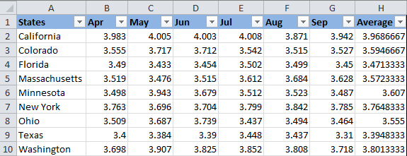
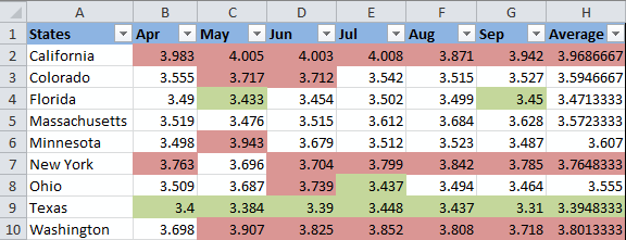
Suppose you have a list of gasoline prices in different states and you want the prices greater than USD 3.7 to be of the color red and equal to or less than USD 3.45 to be of the color green.
Note: The screenshots for this example were captured in Excel 2010, however the buttons, dialogs and settings are the same or nearly the same in Excel 2016 and Excel 2013.
Okay, here is what you do step-by-step:
- Select the table or range where you want to change the background color of cells. In this example, we've selected $B$2:$H$10 (the column names and the first column listing the state names are excluded from the selection).
- Navigate to the Home tab, Styles group, and choose Conditional Formatting > New Rule….

- In the New Formatting Rule dialog box, select "Format only cells that contain" under "Select a Rule Type" box in the upper part of the dialog box.
- In the lower part of the dialog box under "Format Only Cells with section", set the rule conditions. We choose to format only cells with a Cell Value - greater than - 3.7, as you can see in the screenshot below.
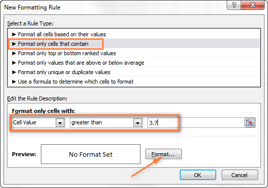
Then click the Format… button to choose what background color to apply when the above condition is met.
- In the Format Cells dialog box, switch to the Fill tab and select the color of your choice, the reddish color in our case, and click OK.
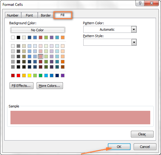
- Now you are back to the New Formatting Rule window and the preview of your format changes is displayed in the Preview box. If everything is Okay, click the OK button.

The result of your formatting will look similar to this:
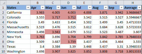
Since we need to apply one more condition, i.e. change the background of cells with values equal to or less than 3.45 to the green color, click the New Rule button again and repeat steps 3 - 6 setting the required condition. Here is the Preview of our second conditional formatting rule:

When you are done, click the OK button. What you have now is a nicely formatted table that lets you see the highest and lowest gas prices across different states at a glance. Lucky they are in Texas :)
Tip: You can use the same method to change the font color based on the cell's value. To do this, simply switch to the Font tab in the Format Cells dialog box that we discussed in step 5 and choose your preferred font color.

How to permanently change a cell's color based on its current value
Once set, the background color will not change no matter how the cell's contents might change in the future.
Task: You want to color a cell based on its current value and wish the background color to remain the same even when the cell value's changes.
Solution: Find all cells with a certain value or values using Excel's Find All function or Select Special Cells add-in, and then change the format of found cells using the Format Cells feature.
This is one of those rare tasks that are not covered in Excel help files, forums and blogs and for which there is no straightforward solution. And this is understandable, because this task is not typical. And still, if you need to change the background color of cells statically i.e. once and forever unless you change it manually again, proceed with the following steps.
Find and select all cells that meet a certain condition
There may be several possible scenarios depending on what kind of values you are looking for.
If you need to color cells with a particular value, e.g. 50, 100 or 3.4, go to the Home tab, Editing group, and click Find Select > Find….

Enter the needed values and click the Find All button.

Tip: Click the Options button in the right-hand part of the Find and Replace dialog to get a number of advanced search options, such as "Match Case" and "Match entire cell content". You can use wildcard characters, such as an asterisk (*) to find any string of characters or a question mark (?) to find any single character.
In our previous example, if we needed to find all gas prices between 3.7 and 3.799, we would specify the following search criteria:

Now select any of the found items in the lower part of the Find and Replace dialog window by clicking on it and then press Ctrl + A to select all found entries. After that click the Close button.

This is how you select all cells with a certain value(s) using the Find All function in Excel.
However, what we actually need is to find all gas prices higher than 3.7 and regrettably Excel's Find and Replace dialog does not allow for such things.
Luckily, there is another tool that can handle such complex conditions. The Select Special Cells add-in lets you find all values in a specified range, e.g. between -1 and 45, get the maximum / minimum value in a column, row or range, find cells by font color, fill color and much more.

You click the Select by Value button on the ribbon and then specify your search criteria on the add-in's pane, in our example we are looking for values greater than 3.7. Click the Select button and in a second you will have a result like this:

If you are interested to try the Select Special Cells add-in, you can download an evaluation version here.
Change the background color of selected cells using "Format Cells" dialog
Now that all cells with a specified value or values are selected (either by using Excel's Find and Replace or Select Special Cells add-in) what is left for you to do is force the background color of selected cells to change when a value changes.
Open the Format Cells dialog by pressing Ctrl + 1 (you can also right click any of selected cells and choose "Format Cells…" from the pop-up menu, or go to Home tab > Cells group > Format > Format Cells…) and make all format changes you want. We will choose to change the background color in orange this time, just for a change :)
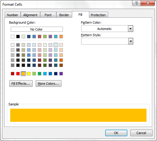
If you want to alter the background color only without any other format changes, then you can simply click the Fill color button and choose the color to your liking.

Here is the result of our format changes in Excel:

Unlike the previous technique with conditional formatting, the background color set in this way will never change again without your notice, no matter how the values change.
Change background color for special cells (blanks, with formula errors)
Like in the previous example, you can change the background color of special cells in two ways, dynamically and statically.
Use Excel formula to change background color of special cells
A cell's color will change automatically based on the cell's value.
This method provides a solution that you will most likely need in 99% of cases, i.e. the background color of cells will change according to the conditions you set.
We are going to use the gas prices table again as an example, but this time a couple of more states are included and some cells are empty. See how you can detect those blank cells and change their background color.
- On the Home tab, in the Styles group, click Conditional Formatting > New Rule… (see step 2 of How to dynamically change a cell color based on value for step-by-step guidance).
- In the "New Formatting Rule" dialog, select the option "Use a formula to determine which cells to format". Then enter one of the following formulas in the "Format values where this formula is true" field:
- =IsBlank()- to change the background color of blank cells.
- =IsError() - to change the background color of cells with formulas that return errors.
Since we are interested in changing the color of empty cells, enter the formula =IsBlank(), then place the cursor between parentheses and click the Collapse Dialog button
 in the right-hand part of the window to select a range of cells, or you can type the range manually, e.g.
 =IsBlank(B2:H12).
- Click the Format… button and choose the needed background color on the Fill tab (for detailed instructions, see step 5 of "How to dynamically change a cell color based on value") and then click OK.
The preview of your conditional formatting rule will look similar to this:

- If you are happy with the color, click the OK button and you'll see the changes immediately applied to your table.

Change the background color of special cells statically
Once changed, the background color will remain the same, regardless of the cell values' changes.
If you want to change the color of blank cells or cells with formula errors permanently, follow this way.
- Select your table or a range and press F5 to open the "Go To" dialog, and then click the "Special…" button.

- In the "Go to Special" dialog box, check the Blanks radio button to select all empty cells.

If you want to highlight cells containing formulas with errors, choose Formulas > Errors. As you can see in the screenshot above, a handful of other options are available to you.
- And finally, change the background of selected cells, or make any other format customizations using the "Format Cells" dialog as described in Changing the background of selected cells.
Just remember that formatting changes made in this way will persist even if your blank cells get filled with data or formula errors are corrected. Of course, it's hard to imagine off the top of the head why someone may want to have it this way, may be just for historical purposes :)
How to get most of Excel and make challenging tasks easy
As an active user of Microsoft Excel, you know that it has plenty of features. Some of them we know and love, others are a complete mystery for an average user and various blogs, including this one, are trying to shed at least some light on them. But! There are a few very common tasks that all of us have to perform daily and Excel simply does not provide any features or tools to automate them or make an inch easier.
For example, if you need to check 2 worksheets for duplicates or merge rows from single or different spreadsheets, it would take a bunch of arcane formulas or macros and still there is no guarantee you would get the accurate results.
That was the reason why a team of our best Excel developers designed and created 70+ add-ins that we call the Ultimate Suite for Excel. These smart tools handle the most grueling, painstaking and error-prone tasks in Excel and ensure quickly, neatly and flawless results. Below is a short list of just some of the tasks the add-ins can help you with:
- Remove duplicates and find unique values
- Merge tables and combine data from different sources
- Combine duplicate rows into one
- Merge cells, rows and columns
- Find and replacing in all data, in all workbooks
- Generate random numbers, passwords and custom lists
- And much, much more.
Just try these add-ins and you will see that your Excel productivity will increase up to 50%, at the very least!
That's all for now. In my next article we will continue to explore this topic further and you will see how you can quickly change the background color of a row based on a cell value. Hope to see you on our blog next week!
 by
by
424 comments
Hello,
I'm trying to set up a sheet where if I enter something in A (will be a number) then B,C,D,E turns red until something is entered into each one.
Once a value, or word is entered in each of B:E they turn back to white.
Is this possible? It seems like trying to connect 2 formulas may be contradicting
I am partially red/green colour blind and rely on the labels that appear when I use Fill on the Home ribbon (pause over a colour and the label appears). But those labels do not appear when I use Fill from the conditional formatting feature. How do I get them to appear when using conditional formatting? Also how do I get labels to appear in 'more colours'?
Hello Kevin,
I am very sorry, I don't know a way to make the labels to appear for conditional formatting colors.
Hi Svetlana
I have a range of values in Row1 - say A1 to J1
I have another range of values in row2 - say A1 to J2.
I am comparing A1 and A2; then B1 with B2....... then J1 to J2.
Whenever value in row1 < row 2, the row2 cell should be changed to red color.
This is needed to be done across the entire row 2.
Kindly let me know the solution.
Hello Sridhar,
If you have to highlight each cell in row 2 that has a value greater than the value in row 1 in the same column, then select row 2 and create a rule with this formula:
=A2>A1
If you have to highlight the entire row 2 if at least 1 cell in row 1 has the value less than in row 2, you need a helper cell, e.g. A5, with the following array formula (remember to press CTRL+Shift+Enter instead of Enter to complete it):
=SUM(--(A1:J1<A2:J2))
After that, select row 2 and create a rule with this formula:
=$A$5>1
Thank you Svetlana!!
Hi,
I have applied conditional formatting to change the color of few cells to red in a row based on a value. After applying conditional formatting,if i copy and paste some data to these cells, the background color changes to white. Can you please help?
Hello Satish,
When you use the standard Paste command, the current rules are replaced with the ones applied to inserted cells.
You need to use the Paste Special option instead: right-click on the destination cells, select Paste Special from the context menu and choose the Values or Formulas radio button under Paste.
Thank you so much, it is very useful!
I also want to create legend after doing these way, how to create leagend?
Thank you indvance!
I am tracking training of people on my project. All of the training they take has to be retaken annually.
Based on the completion date in a cell I want to turn the cell GREEN if the number of days fall within 1 to 334 days from the completion date. I want to turn the cell YELLOW If the number of days fall within 335 to 364 days from the completion date. I want to turn the cell RED if the number of days is 365 or more from the completion date.
In col. B2- 100. In col.A3-101,A4-102,A5-103. In col.C3-99,C4-98,C5-97.
when col.B2 there are 101 i want green color in A3.
when col.B2 there are 102 i want green color in A4.
when col.B2 there are 103 i want green color in A5
& Viseversa
when col.B2 there are 99 i want red color in C3
when col.B2 there are 98 i want red color in C4
when col.B2 there are 97 i want red color in C5
i want to color some selected cells based on cell color
please let me how to do it
Thanks
i want to color selected cell based on cell color
hi the post is very helpful to me bcoz I have learnt a new thing but I got one question how do you do if you want to color the cell after entering the value maybe less than 3 to color yellow and greater than 3 or empty cell to remain with default color
Lets say I have a formula in a cell from another page in the workbook. The cell in the other work book is a drop down. Is there any way when that drop down is used/filled to make the cell on the second page change color to show its populated?
Hello Steph,
It looks like you need a special macro to fulfill this task. I am really sorry we can't help you with this.
Thank you, this topic is helpful
Is there a way to format a column of numbers to highlight only when another column has an "X" in that row?
Hi Patricia,
Of course, there is a way. Simply select the column you want to highlight, not including the header and create a rule for it with this formula:
=A2="X"
Where A2 is the first cell with data in the other column, again not including the header row.
You're the best! Thank you doll
Dear Svetlana Cheusheva,
Can we color a cell based on result. In detail, I am using a formula (=min(various nos of cell in a particular row) to find the lowest figure , Like ( =MIN(W7,S7,O7,K7,like so on))and for example result is W7 cell and I want to automatically color the W7 cell. By conditional formatting it can be done by selecting entire cell range, but problem is I have to more than 40-50 row and I have to repeat the same rule for each row. Is there any help for me. Pls guide.
Hello Rameswar,
You can select all the rows and create the conditional formatting rule with the formula =A7=MIN($W7, $S7, $O7....)
Where A7 is the first (top-left) cell of your range.
But I'd recommend creating a helper column (hidden) and copy the following formula there: =MIN($W7, $S7, $O7....) And in your conditional formatting rule, use the formula =A7=$AB7, where A7 is the top-left column and AB is the helper column.
If you have a large data set, this rule will work much faster because Excel won't have to calculate =MIN($W7, $S7, $O7....) for each cell where the rule is applied.
Thank you for your response, but i might not have explained it well enough.
I have 3 cells that need to change rules according to what i have selected from a drop down list. So, if i have "refrigerator" selected from the list, the 3 cells need to have one rule for that selection, and if i select "freezer" the same 3 cells need to have another set of rules. Not sure how to do it.
Thanks for you help though! :)
Hi Ron,
Regrettably, Excel conditional formatting rules cannot be changed depending on the value selected in the drop down list (this can be done using VBA only).
As an alternative, you can create several rules for the same range of cells, one per each value in the drop-down list, that will check the contents of your drop box and color the cells you want depending on the drop-down list's value and your additional conditions.
Hi,
Can I have a complete row highlighted in any color based on if there is any change (addition or deletion) of data from the exiting value?
Hi Rohit,
You can apply a conditional formatting rule to entire rows. Please see this tutorial for more details - How to change the row color in Excel based on a cell’s value. To be able to suggest a formula, I need more info about your data structure and the result you are looking for.
very nice , thank you.
Please Please Help!!!
My cell C1 has to say "yes" if A1>100 and B1100 and B1>70.
please help how to make this formula ??? My head is broken by now :(
Hi Sergey,
Here you go :)
=IF(AND(A1>100, B1100>70, B1>70),"yes","")
I am creating a task list and I would like to change the fill color of the row depending on to whom the task is assigned. I have created the drop-down list and used conditional formatting to assign colors to the individuals names. Now when I select a name from the drop-down list the fill color changes for that cell. How can I get the corresponding cells in the row to change to the same color?
Hello John,
You just need to apply the rule you created to the entire rows. Please see this tutorial for full details - How to change the row color based on a cell’s value in Excel.
Thank you for taking the time to assist me. It is much appreciated.
i want to color some cells based on different cell's condition. I've done it but the problem is when i close the document after saving and open again then i see that the condition has been erased. but why??
Hi Tanjin,
This is absolutely abnormal! Please make sure you save the workbook after creating the rule.
Sorry, i meant color coded values
Hi Ron,
You can select a group of sells you want to color (e.g. D10:D12) and create 2 rules with different fill colors based on these formulas:
=$D10="Refrigerator" and =$D10="Freezer".
How can you make a group of cells change their rules based on what you select from a drop down list??
I have a drop down list consisting of "Refrigerator" and "Freezer". I have coded values in "D10-D12" that need to change based on whether i have "freezer" or "refrigerator" selected.
Thanks!
Hai,
I have a trend monitoring datasheet . Each kind of trend refers to 1 - 100 numbers. i need to highlight the trend if it occurs more than 2 times.
Eg. Trend No.1 - BY Road, 2 -By shop, 3 -By School ... up to 100 numbers. If trend No.1 occurs two times, it should highlight. Can you please help me.
Hi Anil,
To be able to suggest a proper formula, I need to know more details. Is each trend a column or a row? Do you want to highlight certain cells or entire rows? Please send me a workbook with your sample data at support@ablebits.com and I will try to help.
Hi,
I want to change the cell colors in col A based on the values in another cells say Col C. Here, i have conditions that if the values in Col C are in the range <% then green, if + % then yellow otherwise Red..how to get it done!!
Hi!
You can select all cells with data in column A, not including the column header, and create 3 conditional formatting rules based on the formulas like these (assuming that row 2 is your first row with data).
Green: =$C2<50%
Yellow: =$C2>60%
Red: =AND($C2>=50%,$C2<=60%)
For more details, please check out this tutorial: How to change a cell’s color based on another cell.
I am working with recertification dates of about 100 people. I have columns with recertification dates with an adjacent column that allows me to see if personnel are current or overdue. These cells change color based on that value. Their are several columns of data between the name of the indivual and their status. I would like to highlight names of individuals who are overdue. Is there a way to reference another cell so that when they go overdue it highlights their name and when they return current the highlighting goes away?
Hello Matt,
You can do this by creating a conditional formatting rule based on a formula. Select the column you want to highlight a create a rule using a formula similar to this: =$C2="Overdue" (where C is your status column and 2 is your 1st row with data). You can find more information about conditional formatting based on another cell here: Change a cell’s color based on another cell value.
Hi Svetlana,
I am struggling to figure out how to set a value range in my spreadsheet to correlate with specific colors when a value is input in the cells. For instance, I want the cell color to be blue when the value input into the cells is less or equal to 2.0, and if the value is 3.0 - 4.0 the cell will turn green, and if the value input into the cell is greater than or equal to 4.1 it will turn pink. Can you please help?
Thank you in advance for any assistance you can provide.
Julie
Hi Julie,
You can easily do this by creating 3 separate rules in this way:
- Select all the cells you want to color;
- Click Conditional Formatting > New Rule > Format only cells that contain;
- Select the needed option from the drop-down list (2nd box from the left) for each rule - "less or equal to", "between", and "greater than or equal to";
- Click the Format button and choose the format you want for each rule.
You can find the detailed guidance with screenshots here - Creating an Excel conditional formatting rule. Hopefully you will find the info helpful.
This has been so very helpful. Thank you for sharing your wealth of knowledge. I would love to know how to conditionally format a cell colour based on whether a different cell is NOT blank. I have perfected the blank value, how do I do the opposite?
I am also curious if it is possible to use the icon sets to show based on the value (or the blank versus containing data) of other cells. An example, a check list of items that spans a row, a check mark at the front of the row to show all columns have been filled in (contain data, any data) or an exclamation in the first cell to show that there are some cells that are blank, or an x if all cells in that row are blank. Is that even possible???
Thank you for your time
Hi Michelle,
You can create a rule with the following formula: =$B2="" It will color cells in the selected column(s) if a corresponding cell in Column B is not blank. Naturally, you will need to replace B with the column you need, and "2" with the row number where your data starts.
As for the icon sets, I described a solution exactly for this task in my latest article - How to use conditional formatting in Excel. You can go directly to the section How to apply an icon set based on other cells' values. Hopefully, this is what you are looking for.
Oh my gosh that icon set creativity is brilliant!!! Thanks Svetlana!!
thanks for supporting
How to change colour of entire column ( if > green &if < red)comparison to other column ?
Hello Rasendra,
This is a bit unusual to change the color of the entire column, most other users asked how to change the color of the entire row. Anyway, if this is your task, you can change the color of the whole column in this way:
- Select the entire column, say column B.
- Create 2 rules with these formulas: =$B$2<$A$2 and =$B$2>$A$2 (we are comparing values in row 2).
Make sure both formulas are applied to the entire column, say =$B:$B.
Hi, never mind previous request, I found the answer in another of your articles. Also very good, by the way.
Thank you for your feedback Justine! I am really glad to know you found the articles helpful.
Hi Svetlana, great, easy to understand instruction. I hope I haven't missed this, but I can't see how to color an entire row based on the value in one cell for a whole page of rows. For example - value in A2 is A so row is red, value B makes the row blue, etc. It will take a new rule for each value/color combo? Thanks, Justine
how to fill color by getting two values from two cells respectively.
For ex..
1 2 3 4 5 6 7 8 9
2 6 then from 2nd to 6th column have to fill color.
1 5 then from 1st to 5th column have to fill color.
can u pls help me?
Hi Charu,
I am sorry I do not exactly understand the task. Can you please send us your source data and the desired result at alexander.frolov@ablebits.com? We will try to figure this out.
Hi Svetlana,
Amazingly good post.
I've one question as well.
A3 X
A4 X
A5 Y
A6 Z
A7 Z
A7 X
I'm trying to compare two cells for entire (Current and Preceding) and if they are not equal then fill with some color for the cell which differs from its previous one. I'm using Conditional formatting using a formula - =A2A3
Result is it fills color for A4 instead of A5 and A7 Instead of A8.
Hi Santosh,
Thank you! You simply need to use the cells' addresses in your formula in the reverse order. So, select the needed range, say A3:A8, and create a rule with this formula:
=A3<>A2
That works, Thank You :)
Hi Svetlana,
It's really helpfull article. I appriciate the way you described about the features of Excel.I am working on Excel services using O-data and I am stucked in one point.
Like in given example there are total 10 rows and you did formatting for that.
I want to add 4-5 extra rows in that same sheet.So is there any way that the cells having values greater than 3.7(given in your example) should come in reddish color and cells having values less than or equals tp 3.45(given in your example) should come in green color for extra rows automaticaly without again selecting the entire table.
Hope you can help figure this thing out!
Thanks
Hi Vishesh,
Usually Excel is smart enough to apply the existing conditional formatting rules to the newly added rows. If this does not happen, then you can either:
- When creating a rule, select some more empty rows below your data, say 100 - 200 rows, or
- Convert the range to table (Insert tab > Table). In this case, the existing rules will definitely be applied to all new rows you add to the table.
thanks so much for this useful and well exmapled article, saved me hours on what i was about to do. you're awesome!
Thank you very much, Macca!
HI Svetlana,
Useful post and perfect answers :)
1 Query - i want to format cells in a column with colurs based on the vloopkup value from other sheet.
How can this be acheived?
Hi Adil,
Thank you for your kind words : )
You can use the Vlookup function in the formula, the conditional formatting rules support it. Here is an example:
=VLOOKUP($A2,Lookup!$A$2:$C$100,3)>20
Just keep in mind that Vlookup is a resource-consuming function and it may slow down your Excel if you have large tables.
Dear SC,
Thanks for your article know i know how can i use the conditional formatting for filling the color in an specific column, But could you please tell me how i can fill a color in a specific column based on the value of an another column
With your quoted example how you can color the name of states A1,A2,A3 based on the value of mentioned in the column B1,C1,D1
Hello Radhakrishnan,
You can color the names of states in column A based on values in columns B, C and D in this way:
- Select the cells you want to color (A2:A12 in our example)
- Create a conditional formatting rule based on formula, e.g. =AND($B2<3.5,$C2<3.5,$D2<3.5) It will color the states with gas prices less than 3.5 in columns B - D.
For more information, please check out my other article: How to change a cell's color based on a value of another cell. Hope this helps.
Hi,
For example A1 & B1 both cells values should be same. If it's not true, then C1 cell background need to be change! can you help me?
Hi Saran,
Just select all the cells in column C that you want to change the background color and then create a conditional formatting rule with this formula:
=($A1<>$B1)
I need some help here. I am trying to change the font of Cell A2 red based on B2 being blank. How can I work that out?
Hi,
Select the cells you want to highlight in Column A and create the conditional formatting rule based on this formula: =B2=""
And then choose the needed font color on the Font tab of the Format Cells dialog.
Hi,
I would just like to fill a cell with a color based on a %. Say fill a cell 50% with a color as a graphic representation of the amount. Is that possible in excel?
Thanks
Vinny
Hi Vinny,
Of course, you can do this using the conditional formatting. The easiest way is to select your table or a range of cells, click the Conditional formatting button > Highlight Cells rules > Equal to..., specify the percent you want to color, e.g. 50%, and choose a fill color from the drop down list (click Custom Format... if you want more colors).
Can this be done with a gradient as well? For example setting RED for 0% and GREEN for 100% so it does the colours by itself according to the result of the formula.
I'm using this and I would like the result of this cell to change its colour.
=COUNTIF(E4:E37, "SI")/34
Thank you.
Thanks I was able to find my answer / straight to the point
my problem out side of your presentation
Hello Svetlana,
I'm having a trouble with conditional formatting, I've been looking for solutions several days but still can't figure out.
I use "between" rule to highlight cells. But is there any way that I can highlight cells with 0 and ignore blank cells? Because when I choose highlight between "0" to "46" (for example), blank cells are also highlighted.
I try to use 3-scale color, it can ignore blank cells but unfortunately my data will be much better if I use "between" rule to highlight.
Hope you can help figure this thing out! Thank you very much!!
Best regards!
Hi Thinh,
You can do this by creating a second rule of the "Format only cells that contain" type. In the 'New Formatting rule' dialog window, click the little arrow next to "Cell value" box and choose Blanks from the drop-down list. Then simply click OK without setting any format. Finally, click Conditional Formatting > Manage rule on the ribbon and select the option "Stop if true" next to the Blanks rule. Also, make sure it is first in the list, if not, move it to the top as explained here . Hope this helps : )
Thank you very very much!!! You are such a genius! I've been searching for days with no result! Your solution works exactly as I hope it will!
So much thank you for your help! You've just saved my thesis :)
Best regards!!
I'm glad to know it worked for you. Good luck with your thesis! : )
Hi Svetlana,
Thank you for the post. I have a follow-up question. I have two columns and I want to compare the two values for row 1 in each column for dozens of rows. I want column A's cell to change color if it's value is less than the corresponding cell in Column B. For example if A1=4 and B1=5, then I want A1 to turn red and I want to do this for each cell in A1:A50 compared to each corresponding cell in B1:B50. Is there a way I can do this all at once instead of one cell at a time?
Thanks,
Matt
Hi Matt,
Of course, you can do this at once using the conditional formatting. Select cells A1:A50 and create a new rule (Conditional formatting > New rule > Use a formula to determine which cells to format). Enter this formula =$A1<$B1 and choose the red fill color. Done!
If you want to do the same in a table that has headers (data starts in row 2), then simply change A1 to A2 and B1 to B2 in the formula.
Hi Svetlana,
Thank you, but that only worked for the first cell (assuming I didn't do something wrong). How do I get it to compare A2 to B2 and C2 to C3, etc.? I'm used to using formulas where I could create the formula and then just copy the formula to all of the cells. Is there a similar way to do that with this conditional formatting?
Thanks again,
Matt
Hi Matt,
Yes, it works in a similar way with conditional formatting. Instead of copying the formula to other cells, you select the entire range that you want your formula to apply to, and use a mixed cell reference, i.e. an absolute column and relative row (e.g. $A1 and $B1).
I figured it out. Thanks for your help.
how do you do the above using drop-down menus
Hi Eric,
Sorry, I do not exactly understand your question. I do not know any way to change the background color in Excel other than by using conditional formatting.
it is shorting ....
hi , actually i have 100 cells out of which 10 contains value as 0,
and others are any number ...i have used some formulas , as a result of which 0 value has been entered in the cells,, i want to change the colour of cell containing
0 when its value changes to some new value other then 0, at the same time i do not want to change cell colour of my existing cells containing values other then 0..
pls help
Hi Sameer,
Select your 100 cells, press Ctrl+F, enter 0 into the "Find what" field and click the "Find all" button. Then switch to the list of found values and press Ctrl+A to select them all. After that create a conditional formatting rule by choosing "Format only cells that contain" (the rule will apply to the highlighted cells only). Under "Format only cells with" choose "Cell value", "not equal to", 0. Press the Format button to choose the fill color of your liking and you are done.
great helpfull
i require a range of cells to turn color when the value of a non adjacent cell reaches a specific value, example;
cells b2,b3,b4,b5,b6 to turn red when cell f12 is greater than 20
Hi Gln,
Just select the needed cells (b2:b6) and create a new rule with this formula =$F$12>20.
Hi Dinesh and Hafiz,
Thank you for your comments! It's really nice to know that my article was helpful.
thanks a lot
thanks i found my problem solution.
Its very usefull for me
No i Can't understand
Very easy and Usefull, $nx...