The tutorial explains how to use multiple IF in Excel and provides a couple of nested If formula examples for most common tasks.
If someone asks you what Excel function you use most often, what would your answer be? In most cases, it's the Excel IF function. A regular If formula that tests a single condition is very straightforward and easy to write. But what if your data requires more elaborate logical tests with multiple conditions? In this case, you can include several IF functions in one formula, and these multiple If statements are called Excel Nested IF. The biggest advantage of the nested If statement is that it allows you to check more than one condition and return different values depending on the results of those checks, all in a single formula.
Microsoft Excel has limits to the levels of nested IFs. In Excel 2003 and lower, up to 7 levels were allowed. In Excel 2007 and higher, you can nest up to 64 IF functions in one formula.
Further on in this tutorial, you will find a couple of Excel nested If examples along with a detailed explanation of their syntax and logic.
Example 1. Classic nested IF formula
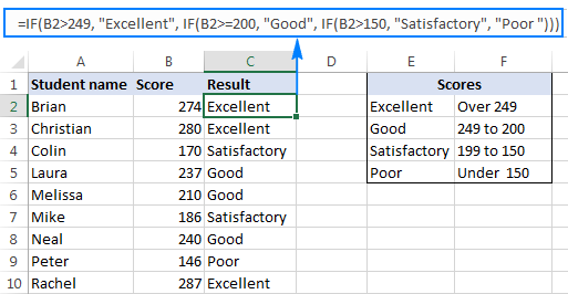
Here's a typical example of Excel If with multiple conditions. Supposing you have a list of students in column A and their exam scores in column B, and you want to classify the scores with the following conditions:
- Excellent: Over 249
- Good: between 249 and 200, inclusive
- Satisfactory: between 199 and 150, inclusive
- Poor: Under 150
And now, let's write a nested IF function based on the above criteria. It's considered a good practice to begin with the most important condition and keep your functions as simple as possible. Our Excel nested IF formula goes as follows:
=IF(B2>249, "Excellent", IF(B2>=200, "Good", IF(B2>150, "Satisfactory", "Poor")))
And works exactly as it should:
Understanding Excel nested IF logic
I've heard some people say that Excel multiple If is driving them crazy :) Try looking at it at a different angle:

What the formula actually tells Excel to do is to evaluate the logical_test of the first IF function and, if the condition is met, return the value supplied in the value_if_true argument. If the condition of the 1st If function is not met, then test the 2nd If statement, and so on.
IF(check if B2>=200, if true - return "Good", or else
IF(check if B2>150, if true - return "Satisfactory", if false -
return "Poor")))
If you need a nested IF formula with wildcard characters (partial match), check out this example: If cell contains, then return different values.
Example 2. Multiple If with arithmetic calculations
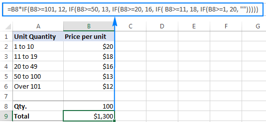
Here's another typical task: the unit price varies depending on the specified quantity, and your goal is to write a formula that calculates the total price for any amount of items input in a specific cell. In other words, your formula needs to check multiple conditions and perform different calculations depending on what amount range the specified quantity falls in:
| Unit Quantity | Price per unit |
| 1 to 10 | $20 |
| 11 to 19 | $18 |
| 20 to 49 | $16 |
| 50 to 100 | $13 |
| Over 101 | $12 |
This task can also be accomplished by using multiple IF functions. The logic is the same as in the above example, the only difference is that you multiply the specified quantity by the value returned by nested IFs (i.e. the corresponding price per unit).
Assuming the user enters the quantity in cell B8, the formula is as follows:
=B8*IF(B8>=101, 12, IF(B8>=50, 13, IF(B8>=20, 16, IF( B8>=11, 18, IF(B8>=1, 20, "")))))
And the result will look something similar to this:
As you understand, this example demonstrates only the general approach, and you can easily customize this nested If function depending on your particular task.
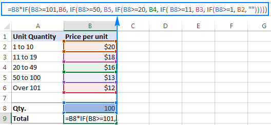
For example, instead of "hard-coding" the prices in the formula, you can reference the cells containing those values (cells B2 to B6). This will enable your users to edit the source data without having to update the formula:
=B8*IF(B8>=101,B6, IF(B8>=50, B5, IF(B8>=20, B4, IF( B8>=11, B3, IF(B8>=1, B2, "")))))
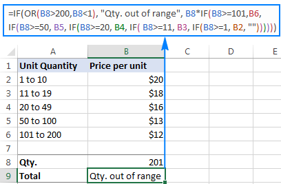
Or, you may want to include an additional IF function(s) that fixes an upper, lower or both bounds of the amount range. When the quantity is outside the range, the formula will display an "out of the range" message. For example:
=IF(OR(B8>200,B8<1), "Qty. out of range", B8*IF(B8>=101,12, IF(B8>=50, 13, IF(B8>=20, 16, IF( B8>=11, 18, IF(B8>=1, 20, ""))))))
The nested IF formulas described above work in all versions of Excel. In Excel 365 and Excel 2021, you can also use the IFS function for the same purpose.
Advanced Excel users that are familiar with array formulas, can use this formula that basically does the same thing as the nested IF function discussed above. Though the array formula is far more difficult to comprehend, let along to write, it has one indisputable advantage - you specify the range of cells containing your conditions rather than referencing each condition individually. This makes the formula more flexible, and if your users happen to change any of the existing conditions or add a new one, you will only have to update a single range reference in the formula.
Excel nested IF - tips and tricks
As you have just seen, there is no rocket science in using multiple IF in Excel. The following tips will help you improve your nested IF formulas and prevent common mistakes.
Nested IF limits
In Excel 2007 - Excel 365, you can nest up to 64 IF functions. In older versions of Excel 2003 and lower, up to 7 nested IF functions can be used. However, the fact that you can nest a lot of IFs in one formula doesn't mean you should. Please keep in mind that each additional level makes your formula more difficult to understand and troubleshoot. If your formula has too many nested levels, you may want to optimize it by using one of these alternatives.
The order of nested IF functions matters
The Excel nested IF function evaluates the logical tests in the order they appear in the formula, and as soon as one of the conditions evaluates to TRUE, the subsequent conditions are not tested. In other words, the formula stops after the first TRUE result.
Let's see how it works in practice. With B2 equal to 274, the nested IF formula below evaluates the first logical test (B2>249), and returns "Excellent" because this logical test is TRUE:
=IF(B2>249, "Excellent", IF(B2>=200, "Good", IF(B2>150, "Satisfactory", "Poor")))
Now, let's reverse the order of IF functions:
=IF(B2>150, "Satisfactory", IF(B2>200, "Good", IF(B2>249, "Excellent", "Poor")))
The formula tests the first condition, and because 274 is greater than 150, the result of this logical test is also TRUE. Consequently, the formula returns "Satisfactory" without testing other conditions.
You see, changing the order of IF functions changes the result:

Evaluate the formula logic
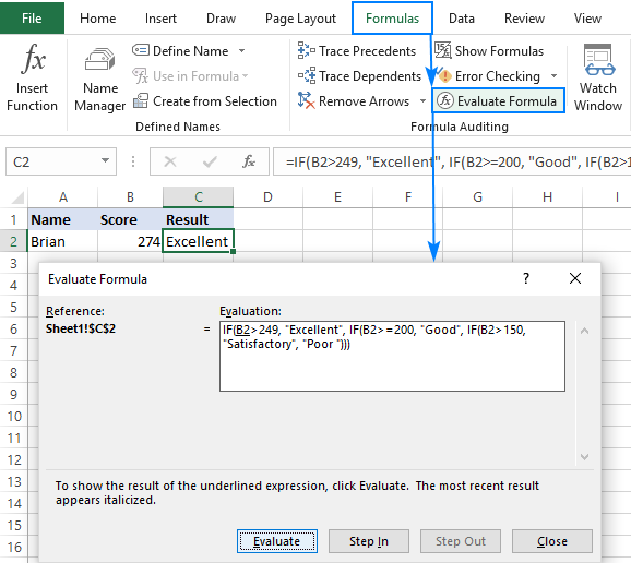
To watch the logical flow of your nested IF formula step-by-step, use the Evaluate Formula feature located on the Formula tab, in the Formula Auditing group. The underlined expression is the part currently under evaluation, and clicking the Evaluate button will show you all the steps in the evaluation process.
For example, the evaluation of the first logical test of the nested IF formula shown in the screenshot below will go as follows: B2>249; 274>249; TRUE; Excellent.
Balance the parenthesis of nested IF functions
One of the main challenges with nested IFs in Excel is matching parenthesis pairs. If the parentheses do not match, your formula won't work. Luckily, Microsoft Excel provides a couple of features that can help you to balance the parentheses when editing a formula:
- If you have more than one set of parentheses, the parenthesis pairs are shaded in different colors so that the opening parenthesis matches the closing one.
- When you close a parenthesis, Excel briefly highlights the matching pair. The same bolding, or "flickering", effect is produced when you move through the formula by using the arrow keys.

For more information, please see Match parenthesis pairs in Excel formulas.
Treat text and numbers differently
When building logical tests of your nested IF formulas, remember that text and numbers should be treated differently - always enclose text values in double quotes, but never put quotes around numbers:
Right: =IF(B2>249, "Excellent",…)
Wrong: =IF(B2>"249", "Excellent",…)
The logical test of the second formula will return FALSE even if the value in B2 is greater than 249. Why? Because 249 is a number and "249" is a numeric string, which are two different things.
Add spaces or line breaks to make nested IFs easier to read
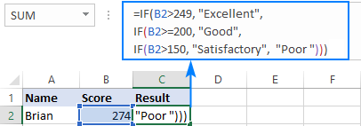
When building a formula with multiple nested IF levels, you can make the formula's logic clearer by separating different IF functions with spaces or line breaks. Excel doesn't care about extra spacing in a formula, so you may not worry about mangling it.
To move a certain part of the formula to the next line, just click where you want to insert a line break, and press Alt + Enter. Then, expand the formula bar as much as needed and you will see that your nested IF formula has become much easier to understand.
Alternatives to nested IF in Excel
To get around the limit of seven nested IF functions in Excel 2003 and older versions and to make your formulas more compact and fast, consider using the following alternatives to nested Excel IF functions.
- To test multiple conditions and return different values based on the results of those tests, you can use the CHOOSE function instead of nested IFs.
- Build a reference table and a use VLOOKUP with approximate match as shown in this example: VLOOKUP instead of nested IF in Excel.
- Use IF with logical functions OR / AND, as demonstrated in the these examples.
- Use an array formula like shown in this example.
- Combine multiple IF statements by using the CONCATENATE function or the concatenate operator (&). A formula example can be found here.
- For experienced Excel users, the best alternative to using multiple nested IF functions might be creating a custom worksheet function using VBA.
This is how you use an If formula in Excel with multiple conditions. I thank you for reading and hope to see you on our blog next week.
Practice workbook for download
Nested If Excel statements (.xlsx file)
 by
by
635 comments
Hi, Ms. Svetlana Cheusheva,
Your artile about IF condition really nice, can help me out for below data style, what will I apply formula for this to get better result (there are 3 Conditions to check);
PROJECT # TRAVEL TYPE DI STATUS COST CODE REMARKS
CONDITION 1 CONDITION 2 CONDITION 3
8326 LEAVE DIRECT TQ.08326-VC-L
8326 LEAVE INDIRECT TQ.08326-FC-I
8326 MOB DIRECT TQ.08326-VC-O
8326 MOB INDIRECT TQ.08326-FC-O
8326 OFFICIALTRAVEL DIRECT TQ.08326-VC-V
8326 OFFICIALTRAVEL INDIRECT TQ.08326-FC-V
RESULT TO BE REQUIRED IN FINAL SHEET AS BELOW;
FOR EXAMPLE
IF PROJECT # "8326" AND "LEAVE" AND "DIRECT" THEN CODE PASTE "TQ.08326-VC-L" IN REQUIRED COLUMN
Your prompt and favorable response will be highly appriciated.
Thanks & regards,
Riz
hello,
very helpful website...
I ve a query, I m looking to use IFERROR for more than 2 conditions with formula as pr below
=IFERROR(VLOOKUP(F2,'Formula report'!B:I,8,FALSE),dxg(F2,"XXX",,"XXXX Days")*100),=IFERROR(VLOOKUP(F2,'Formula report'!B:I,8,FALSE),dxg(F2,"VWAF",,"YYY: 7 Days")*100), "NO DATA"
Does someone is able to help me ?
ty
rene
Hello,
Here is the Data/Table(Sheet1)
ColumnA = Product Name
ColumnB = Amount
ColumnC = Barcode
**more or less there's 25-30 items in each given Column**
Is there a formula where in once barcode has been inputted/coded, ProductName and Amount will came after. (Sheet2)
Hello, I am trying to use nested IF formula including OR, without success. This is what I'm looking for:
Currently my data includes a column of "PASS"/"FAIL" results for each type of test, one Math and one Lit. I just need to identify which tests were taken based on whether or not results are present. Blank cells indicate a test was not taken. With the specific text of "Math + Lit" when indicating both tests were taken.
Example:
MATH LIT TAKEN
Pass Pass Math + Lit
Fail Pass Math + Lit
Fail Math
Fail Lit
Pass Math
Pass Fail Math + Lit
Pass Lit
Fail Fail Math + Lit
In cell D3, enter a nested IF function that will check
cell B3. If B3 is 120 or less, display the text string "Normal", IF B3 is greater than 120,
have Excel check B3 to see if it greater than 139. If it is greater than 139, it should
display the text string "High". If it is greater than 120 but less than 140, it should display
the text string "Prehypertensive".
20. Copy the formula down the whole column through 7/31 Can someone help me please!!!!!!
column A - 10000
column B - % (=E/A)
column c - wk1-8000
column d - wk2-7000
column e - wk3-6000
Is there a formula that I can auto update column B instead of manual update every week.
A B C D E F
Plant 10,000 Target Inv % 8000 7000 6000
Is there a way to create a formula in column c to auto update the % base on the current week. Instead of manual update column C weekly (=F/B and the next week G/B).
Hi,
I need multiple if condition to be merged.
Condition:
if A1= "implementation" & A2= "Complete" & A3="Complete"
Output should be:"Well Done"
if A1= "implementation" & A2= "NA" & A3="Complete"
Output : "Check ABC"
if A1= "implementation" & A2= "Complete" & A3="NA"
Output : "Check XYZ"
if A1= "implementation" & A2= "NA" & A3="NA"
Output : "Incorrect Processing"
I want these outputs if above conditions(inputs) are placed in the 3 cells. can it be done?
Let me know and please email to personal id if possible.
Hello,
I am trying to create a formula where I have 4 Yes/No fields but only 3 Yes's are required to obtain a final yes. I am having trouble figuring out how to write a formula where 3 of 4 yes's = final YES.
As you can tell, I am no excel expert so help is appreciated.
Thank you
L3 Yes/No
O3 Yes/No
R3 Yes/No
U3 Yes/No
These cells are the results of someone meeting a subset of criteria so there will be a yes if the criteria is met or a no if it is not. Same for all of the above cells. To fulfill the whole set of criteria, there must be 3 out of 4 Yeses. V3 will be either "Yes" the criteria has been met or "No" it has not been met.
I hope that helps.
I'm trying to make the formula return 4 possible answer which is (R-regular,A-absent,L-late,OT-overtime). My basis for regular is if the value of the cell is "8". So this is the formula that I made so far =IF(H16>7.9,"OT",IF(H16<7.9,"L",IF(H16=8,"R","A"))). It only returns (OT and L) something is very wrong and i can't figure it out. I'm just new to excel so please help me. Thank you so much in advance
I'm trying to make the formula return 4 possible answer which is (R-regular,A-absent,L-late,OT-overtime). My basis for regular is if the value of the cell is "8". So this is the formula that I made so far =IF(H16>7.9,"OT",IF(H16<7.9,"L",IF(H16=8,"R","A"))). It only returns (OT and L) something is very wrong and i can't figure it out. I'm just new to excel so please help me
Hi, I make a sheet for distribution incentive . her have multiple uneven amount . I want of use ceiling & floor e formula in on cell. How i use this formula ? i want to bellow this type to use by formula.
previous Required/Revised amount
amount
11,957 12,000 (IF Above 500 + it will next round amount
18,396 18,000 IF below -500 it will Previous round amount
7,818 8,500 (IF Above 500 + it will nearest round amount
7,818 7,500
5,059 5,000
Hi, I am trying to modify a current if/then combined calculation statement to reflect the proper calculation. Here is the original:
IIF (UDField09 < 86666.67, IIF (UPPER(last(2,TRIM(PayGroup)))='WK',
UDField09*.26627, UDField09*.576923), IIF (UPPER(last(2,TRIM(PayGroup)))='WK',23076.93,50000))
What I ultimately want it to do in the calc is this. I know I need some nesting and that is where I am having trouble. How should the 3rd line read?
IIF(UDField09 < 86666.67, IIF (UPPER(last(2,TRIM(PayGroup)))='WK',
UDField9/52/10*.36*12/52, UDField9/24/10*.36*12/52, IIF (UPPER(last(2,TRIM(PayGroup)))='WK',23076.93,50000))
I have a file containing multiple sheets the first of which is an index
sheet. The other sheets are hidden. I want to be able to click on a
hyperlink in the index sheet that will send me to the hidden sheet and
open it.
Is this possible ?
I have been trying to fix this formula all day, I don't know at this point what I'm doing wrong.
=IF(D2=Full,A2=1, IF(D2=Special Case, A2=2,IF(D2=Parts, A2=3,IF(D2=T&M, A2=4,IF(D2=Not Installed,A2=5, IF(D2=Customer Issue, A2=6))))))
Please help!
Hi Erika,
If my understanding is correct, you want the output in cell A2. If so, you should not reference A2 in the formula, just enter the formula in the target cell:
=IF(D2="Full", 1, IF(D2="Special Case", 2,IF(D2="Parts", 3, IF(D2="T&M", 4, IF(D2="Not Installed", 5, IF(D2="Customer Issue", 6, ""))))))
Also, please pay attention that all text values should be enclosed in double quotes.
I have 16K+ line items and I am trying to create a formula to take out manual work that will take hours. My forumla is below. The message I get in the cell is#NAME?
What am I doing wrong?
=IF(B297=ZRO,"Return Order", IF(B297=ZC2,"Credit Request", IF(B297=ZD2,"Debit Request", IF(B297=ZB3, "Incentives", IF(B297=ZB4,"Incentives")))))
Hi Alice,
The problem is in the logical text of the first IF (B297=ZRO). "ZRO" is a text value, so it should be enclosed in double quotes (as well as "ZC2", "ZD2", etc. if they are text). If these are cell references, no double quotes then, but you need to fix ZRO anyway.
HI, wonder if I could get help writing a function or direct me to a resource it would help me formulate it myself:
A1 * (B1 or C1 when B1 or C1 is different from zero or different from 'blank')
The B1 OR C1 values will be attributed from a pull down menu and it will be either B1 or C1). It seems so simple and easy but I have almost burned my brains out and nothing!
Thanks a million!!!
Hello,
I'm trying to use nested if with the following syntax but it keeps give me value error
=IF(LEFT(B5,4)="0122","Orange"), IF(LEFT(B5,4)="0127","Orange"), IF(LEFT(B5,4)="0120","Orange"), IF(LEFT(B5,4)="0128","Orange"))))
can you help me please
thanks
Can anyone help me with the argument below.
Age exceeding 10yrs but less than 12yrs - 5%
Age exceeding 12yrs but less than 15yrs - 20%
Age exceeding 15yrs - 50%
Assuming if Cell D3 is between 10 -12 = 5%, Cell D3 if greater than 12 but less than 15 = 20% and if greater 15 = 50%
I want to put the IF formula in Cell E10
If D3 12 but 15 then 50%
Thanks in advance
Hello. Thank you for contacting us.
Please try the following formula to get the result you need:
=IF(D3>=15, "50%", IF(D3>=12, "20%", IF(D3>=10, "5%", "")))
Thank soo much
I want a cell C6 to perform this function -
IF cell g2 falls between 45282 and 90563 then take g2 and subtract it by 45282 multiplied by .335.
If cell g2 is greater than 90563, simply do 45281 multiplied by .335.
How would I write this? Possible? Any help would be appreciated, thanks.
Afternoon,
I have a status column (Column B) that I would like to display "Open", "Closed", "Hold" or "Rejected" based on the contents of another column (Column N) in the same worksheet.
Open would be anything where Column N is blank
Closed would be anything where Column N contains a date
Hold would be anything where Column N has the word "HOLD"
Rejected would be anything where Column N has the word "Rejected"
Many thanks in advance
"# of Service
Provided" Fair
59 61%
108 61%
112 60%
123 63%
134 63%
147 68%
156 71%
I am trying to to put a formula if # of service provided 100 & 110 & 120&130&140 then add 3% with the fair column
I want a bill format like if quantity is 1 then discount will be 40% of amount and if quantity is 2 then discount will be 50% of the total amount and if quantity is 3 then discount will be 60% of the total amount
Hello, Jai,
Thank you for contacting us.
You may try the formula below:
=IF(D2=1, "40%", IF(D2=2, "50%", IF(D2=3, "60%", " ")))
I hope this helps. Please let me know if you have any other questions or difficulties.
I want set multiple condition in on cell below mention in brief
For male professional tax
7501 to 10000 then 175
Above 10000 then 200
For Feb month 300
For Female
Below 10000 then 0
Above 10000 then 200
For feb month 300
Hi everybody!!!
I want one formula for below problem.
Distance 0-50 kg 51-100 kg 101-250 kg 251-500 kg
Upto 25 NIL NIL NIL NIL
26-100 km 650 750 1000 1150
101-150 km 1000 1250 1500 1750
151-200 km 1250 1500 1750 2000
201-300 km 1500 1750 2000 2500
I mention here my dada. Sorry I am unable to give in excel.
I required formula for 2 condition i.e.
Distance 100 km & weight 50 kg = 650
Distance 100 km & weight 100 kg = 750 (2nd condition change)
Distance 100 km & weight 250 kg = 1000 (2nd condition change)
distance 100 km & weight 500 kg = 1150 (2nd condition change)
same with distance 150 to 300 km & weight 50 to 500 kg
I tried 'if and' formula but it's not working multiple time. Please help..
Hi, thanks for this great site. I am stumped with an Excel nested if that uses SEARCH to query for text in the adjoining column. Here's an example
=IF(SEARCH("a",A1),"A",IF(SEARCH("b",A1),"B",IF(SEARCH("c",A1),"C",IF(SEARCH("d",A1),"D",IF(SEARCH("e",A1),"E","other")))))
Unfortunately, I only get "A" or "#VALUE". I tried including IFERROR but got the same results
=IFERROR(IF(SEARCH("a",A1),"A",IF(SEARCH("b",A1),"B",IF(SEARCH("c",A1),"C",IF(SEARCH("d",A1),"D",IF(SEARCH("e",A1),"E"))))),"other")
This only returns "A" or "other". Can you please explain why my nested loop is not nesting? Thanks in advance.
FYI, I first thought the formula was chopped off but then realized that you have to side-scroll to see the entire line.
Hi Need your help,
I need a formula where:
If both x & y exist in column A it will show "Yes" in column C
IF only x or y exist in column A (not both) it will show No in column C
and if both does not exist in column a it will show None in column C.
Thank you!
I am trying to find a formula that will allow me to add a certain number of days to a date in a cell, dependent on certain information in another cell. For example:
A1 B1 C1
Date Rcv'd Level Date Response Due
6/30/17 Level 1 A1 + 20 days if Level 1
A1 + 30 days if Level 2
A1 + 30 days if Level 3
When I tried, I couldn't get the formula to recognize A1 as a date.
Thank you for your time and consideration in this matter. Any assistance would be greatly appreciated.
Hi all,
I'm hoping someone can help me please. I am trying to set up my own manufacturing schedule that shows products, volumes, times and dates etc. I have a formula that works out how long any given production run will take but I want to also take into account the change overs between products.
So, column C is drop down menu with all products and change overs, column E works out how many hours the run will take - I need a formula that looks to column C to see if it shows "change over 10" or "change over 30" and then returns 10 or 30 respectively - if neither are shown then run the calculation (D10/34/60)......
Is this possible? Thanks in advance for any help :)
how to hyperlink in a cell according to condition to open different - different data.
how to open excel sheet with drop down list; or combo box
Hi
I am trying to below pull below output on conditions A B & C, could you please help me in this (if B = C then based on column A it should extract the output)
Column A B C Output
Transactions No Yes Client custom in both versions > Transactions
Accounts No Yes Client custom in both versions > Accounts
No Yes Client custom in both versions
Cotains "History" No No This metadata appears only in V7 client database. Newly added metadata item under "History" folder.
Cotains "1000INT BE" No No Interest BE added in V7
Yes No New Standard Data item
Yes Yes 712 Metadata items match with both 61 and 712 Standard Template
why and how of a bracket {} in this IF argument:
{=MAX(IF('C6'!C:C<=WorkEx!I21,'C6'!C:C))}
The formulae result is different with and without bracket. Thank you.
Hi! I need help with my excel formula. I currently have conditions set on 1 cell. However, how do you add one more condition so that when you input a value on the other cell, the value on the current cell which has the formulas change? Help please please please
Hi,
I am trying to get the OT time and Regular working Hours both in different cells with below formula but the result value is something different, please help?
For Regular working hours =IF((((C6-B6)+(E6-D6))*24)>8,8,((C6-B6)+(E6-D6))*24) and for OT =IF(((C6-B6)+(E6-D6))*24>8, ((C6-B6)+(E6-D6))*24-8,0) , where column B is Log in, column C is Lunch Starts, column D is Lunch Ends and column E is Log Out.
Hi,
I am trying to get the OT time and Regular working Hours both in different cells with below formula but the result value is something different, please help?
For Regular working hours =IF((((C6-B6)+(E6-D6))*24)>8,8,((C6-B6)+(E6-D6))*24) and for OT =IF(((C6-B6)+(E6-D6))*24>8, ((C6-B6)+(E6-D6))*24-8,0)
please send me the file my email id because i am able see your share file
Can we change case of text in excel without use change case formula (Uppercase, lower case, proper case)
You need a macro to do so. A function can only return a value in excel.
I can share the Macro file! Share your mail id.
By this you only need to select the range and Alt+F8.
i need help for below :
If forth character of cell A1 is C and forth character of cell b1 is C then i need reply 2 in cell C1, if forth character of cell A1 is P and forth character of cell b1 is C then i need reply 1 in cell C1, if forth character of cell A1 is P or C and forth character of cell b1 is H then i need reply 5 in cell C1, please help
Thanks
Sanjay Goyal
=IF(E18>TIME(9,10,0),"A",IF(E18>TIME(15,10,0),"A",IF(E18>TIME(21,10,0),"A","P")))
whats wrong in this formula
my calculation attendance time such as 9:10>Late, 15:10>Late, 21:10 Late,or <less then Present
plz help me formula
Hi
I wanna to add time condition with stock price
Like
Open Ltp Time
223 223 9:15
Now i need if open=ltp at 9:15 then it print good to enter else blank
as Ltp is dynamic so i wanna to capture values at 9:15 only.
Hope for early and quick response
Thanks in advance
I need to create an IF..AND formula for these conditions:
calculate the total cost of the car rental (#days * cost)
if the transaction is eligible, give a 20% discount on #days * cost
if the transaction chose to add gas,add $65
So the possible outcomes are:
days * cost only
days * cost minus discount
days * cost plus gas
days * cost minus discount plus gas.
I have been banging my head for too long. I know it needs to be nested, but...
Thank you
This formula returns #VALUE.
=IF(AND('Maint Pricing'!$B2="Flat Rate",'Monthly Calculation'!$D4="Yes"),('Maint Pricing'!$X2+'Maint Pricing'!$Q2),'Maint Pricing'!$X2), IF(AND('Maint Pricing'!$B2="Area Rate",'Monthly Calculation'!$D4="Yes"),('Maint Pricing'!$V2+'Maint Pricing'!$Q2),'Maint Pricing'!$V2)
Can someone help me with this?
Need your help with a formula.
I need to subtract the percentage of a value based on the number of items selected.
The percentages need to change based on the number of items selected.
Exeample> one item costs 10 usd.
take 1 item 0% take 2 items 15%bonus, take 3to5 items 30% bonus take 6to10 50% bonus.
I want to be able to select the number of items in a cell, and in another cell show the value according to the number of items selected.
Can someone help me?
Hello,
I'm bit confuse in applying "If" formula to my data, where I want to get data by applying specific condition;
I want data like, "If Employee X has completed any Job in Task1 then he will get XYZ Units, same way, if Employee X has completed Job in Task2 than he will get ABC Units.
So I'm bit confused what formula to use here, could you please guide me here?
Thanks,
Milan
I am trying to set up a formula were New=New, Used_Like_New=Like New, Used_Very_Good=Very Good, Used_Good=Good, & Used_Acceptable=Acceptable.
The formula I tried was =IF(AND(G2>=New), "New", "" & IF(AND(G2>=Used_Like_New), "Like New", "" & IF(AND(G2>=Used_Very_Good), "Very Good", "" & IF(AND(G2>=Used_Good), "Good ", "" & IF(AND(G2>=Used_Acceptable), "Acceptable", ""))))). I also tried =IF(AND(G2=New), "New", "" & IF(AND(G2=Used_Like_New), "Like New", "" & IF(AND(G2=Used_Very_Good), "Very Good", "" & IF(AND(G2=Used_Good), "Good ", "" & IF(AND(G2=Used_Acceptable), "Acceptable", ""))))).
I have had no luck. This is my first attempt at an If formula. Can you help me out here?
Hi Chris,
Here's the correct syntax:
=IF(G2="New", "New", IF(G2="Used_Like_New", "Like New", IF(G2="Used_Very_Good", "Very Good", IF(G2="Used_Good", "Good ", IF(G2="Used_Acceptable", "Acceptable", "")))))
Thank you!!!
Not sure why my last post didnt include my actual formula but since its not working its not a biggy :)
Hi Milli,
Our blog engine occasionally mangles formulas in comments, sorry for that.
As for your formula, please try this one:
=IF(E3="", "", IF(E3<=1989, 1, IF(E3<=2013, 2, "")))
If the list separator in your Regional Settings is set to semicolon, then it should be written like this:
=IF(E3=""; ""; IF(E3<=1989; 1; IF(E3<=2013; 2; "")))
Please note that the formula will return nothing (an empty string) if E3 is greater than 2013.
Hello!
Not sure why excel hates my If formula...
Point is- if a cell value (let's say "E3") is missing, do nothing. if it's smaller than 1989, write 1, if its between 1990 and 2013, write 2.
I wrote : if ((0>E3E3<2013);2))
but its not working :-(
Would be grateful for your advice!
M.
Hi, in column B i have date & column C other commodity and I want to calculate on basis of date can any one help.
Hi, i have one question plz guide me, i have tow columns with same values, i used if I5 is less than one get H5 value, but the result is not comimg what i want
=if(I5<1,"=H5")
Can you help me.
Thanks