The tutorial explains how to use multiple IF in Excel and provides a couple of nested If formula examples for most common tasks.
If someone asks you what Excel function you use most often, what would your answer be? In most cases, it's the Excel IF function. A regular If formula that tests a single condition is very straightforward and easy to write. But what if your data requires more elaborate logical tests with multiple conditions? In this case, you can include several IF functions in one formula, and these multiple If statements are called Excel Nested IF. The biggest advantage of the nested If statement is that it allows you to check more than one condition and return different values depending on the results of those checks, all in a single formula.
Microsoft Excel has limits to the levels of nested IFs. In Excel 2003 and lower, up to 7 levels were allowed. In Excel 2007 and higher, you can nest up to 64 IF functions in one formula.
Further on in this tutorial, you will find a couple of Excel nested If examples along with a detailed explanation of their syntax and logic.
Example 1. Classic nested IF formula
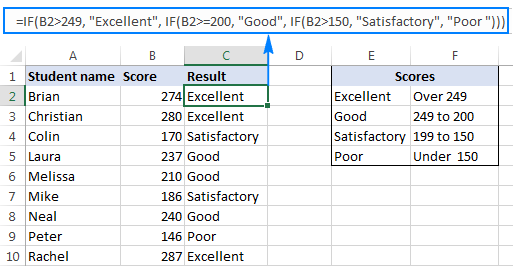
Here's a typical example of Excel If with multiple conditions. Supposing you have a list of students in column A and their exam scores in column B, and you want to classify the scores with the following conditions:
- Excellent: Over 249
- Good: between 249 and 200, inclusive
- Satisfactory: between 199 and 150, inclusive
- Poor: Under 150
And now, let's write a nested IF function based on the above criteria. It's considered a good practice to begin with the most important condition and keep your functions as simple as possible. Our Excel nested IF formula goes as follows:
=IF(B2>249, "Excellent", IF(B2>=200, "Good", IF(B2>150, "Satisfactory", "Poor")))
And works exactly as it should:
Understanding Excel nested IF logic
I've heard some people say that Excel multiple If is driving them crazy :) Try looking at it at a different angle:

What the formula actually tells Excel to do is to evaluate the logical_test of the first IF function and, if the condition is met, return the value supplied in the value_if_true argument. If the condition of the 1st If function is not met, then test the 2nd If statement, and so on.
IF(check if B2>=200, if true - return "Good", or else
IF(check if B2>150, if true - return "Satisfactory", if false -
return "Poor")))
If you need a nested IF formula with wildcard characters (partial match), check out this example: If cell contains, then return different values.
Example 2. Multiple If with arithmetic calculations
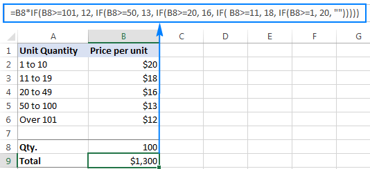
Here's another typical task: the unit price varies depending on the specified quantity, and your goal is to write a formula that calculates the total price for any amount of items input in a specific cell. In other words, your formula needs to check multiple conditions and perform different calculations depending on what amount range the specified quantity falls in:
| Unit Quantity | Price per unit |
| 1 to 10 | $20 |
| 11 to 19 | $18 |
| 20 to 49 | $16 |
| 50 to 100 | $13 |
| Over 101 | $12 |
This task can also be accomplished by using multiple IF functions. The logic is the same as in the above example, the only difference is that you multiply the specified quantity by the value returned by nested IFs (i.e. the corresponding price per unit).
Assuming the user enters the quantity in cell B8, the formula is as follows:
=B8*IF(B8>=101, 12, IF(B8>=50, 13, IF(B8>=20, 16, IF( B8>=11, 18, IF(B8>=1, 20, "")))))
And the result will look something similar to this:
As you understand, this example demonstrates only the general approach, and you can easily customize this nested If function depending on your particular task.
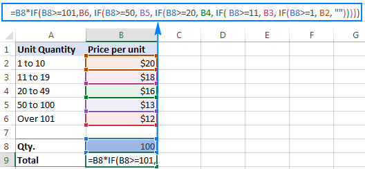
For example, instead of "hard-coding" the prices in the formula, you can reference the cells containing those values (cells B2 to B6). This will enable your users to edit the source data without having to update the formula:
=B8*IF(B8>=101,B6, IF(B8>=50, B5, IF(B8>=20, B4, IF( B8>=11, B3, IF(B8>=1, B2, "")))))
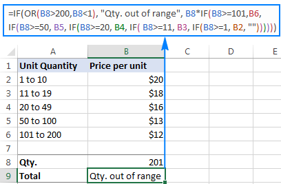
Or, you may want to include an additional IF function(s) that fixes an upper, lower or both bounds of the amount range. When the quantity is outside the range, the formula will display an "out of the range" message. For example:
=IF(OR(B8>200,B8<1), "Qty. out of range", B8*IF(B8>=101,12, IF(B8>=50, 13, IF(B8>=20, 16, IF( B8>=11, 18, IF(B8>=1, 20, ""))))))
The nested IF formulas described above work in all versions of Excel. In Excel 365 and Excel 2021, you can also use the IFS function for the same purpose.
Advanced Excel users that are familiar with array formulas, can use this formula that basically does the same thing as the nested IF function discussed above. Though the array formula is far more difficult to comprehend, let along to write, it has one indisputable advantage - you specify the range of cells containing your conditions rather than referencing each condition individually. This makes the formula more flexible, and if your users happen to change any of the existing conditions or add a new one, you will only have to update a single range reference in the formula.
Excel nested IF - tips and tricks
As you have just seen, there is no rocket science in using multiple IF in Excel. The following tips will help you improve your nested IF formulas and prevent common mistakes.
Nested IF limits
In Excel 2007 - Excel 365, you can nest up to 64 IF functions. In older versions of Excel 2003 and lower, up to 7 nested IF functions can be used. However, the fact that you can nest a lot of IFs in one formula doesn't mean you should. Please keep in mind that each additional level makes your formula more difficult to understand and troubleshoot. If your formula has too many nested levels, you may want to optimize it by using one of these alternatives.
The order of nested IF functions matters
The Excel nested IF function evaluates the logical tests in the order they appear in the formula, and as soon as one of the conditions evaluates to TRUE, the subsequent conditions are not tested. In other words, the formula stops after the first TRUE result.
Let's see how it works in practice. With B2 equal to 274, the nested IF formula below evaluates the first logical test (B2>249), and returns "Excellent" because this logical test is TRUE:
=IF(B2>249, "Excellent", IF(B2>=200, "Good", IF(B2>150, "Satisfactory", "Poor")))
Now, let's reverse the order of IF functions:
=IF(B2>150, "Satisfactory", IF(B2>200, "Good", IF(B2>249, "Excellent", "Poor")))
The formula tests the first condition, and because 274 is greater than 150, the result of this logical test is also TRUE. Consequently, the formula returns "Satisfactory" without testing other conditions.
You see, changing the order of IF functions changes the result:

Evaluate the formula logic
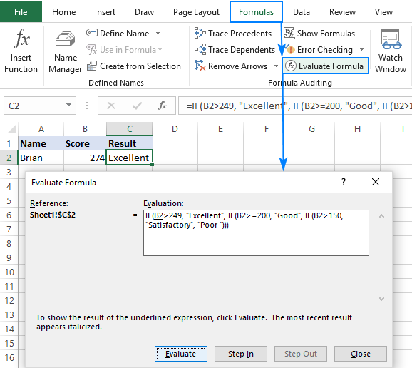
To watch the logical flow of your nested IF formula step-by-step, use the Evaluate Formula feature located on the Formula tab, in the Formula Auditing group. The underlined expression is the part currently under evaluation, and clicking the Evaluate button will show you all the steps in the evaluation process.
For example, the evaluation of the first logical test of the nested IF formula shown in the screenshot below will go as follows: B2>249; 274>249; TRUE; Excellent.
Balance the parenthesis of nested IF functions
One of the main challenges with nested IFs in Excel is matching parenthesis pairs. If the parentheses do not match, your formula won't work. Luckily, Microsoft Excel provides a couple of features that can help you to balance the parentheses when editing a formula:
- If you have more than one set of parentheses, the parenthesis pairs are shaded in different colors so that the opening parenthesis matches the closing one.
- When you close a parenthesis, Excel briefly highlights the matching pair. The same bolding, or "flickering", effect is produced when you move through the formula by using the arrow keys.

For more information, please see Match parenthesis pairs in Excel formulas.
Treat text and numbers differently
When building logical tests of your nested IF formulas, remember that text and numbers should be treated differently - always enclose text values in double quotes, but never put quotes around numbers:
Right: =IF(B2>249, "Excellent",…)
Wrong: =IF(B2>"249", "Excellent",…)
The logical test of the second formula will return FALSE even if the value in B2 is greater than 249. Why? Because 249 is a number and "249" is a numeric string, which are two different things.
Add spaces or line breaks to make nested IFs easier to read
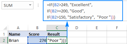
When building a formula with multiple nested IF levels, you can make the formula's logic clearer by separating different IF functions with spaces or line breaks. Excel doesn't care about extra spacing in a formula, so you may not worry about mangling it.
To move a certain part of the formula to the next line, just click where you want to insert a line break, and press Alt + Enter. Then, expand the formula bar as much as needed and you will see that your nested IF formula has become much easier to understand.
Alternatives to nested IF in Excel
To get around the limit of seven nested IF functions in Excel 2003 and older versions and to make your formulas more compact and fast, consider using the following alternatives to nested Excel IF functions.
- To test multiple conditions and return different values based on the results of those tests, you can use the CHOOSE function instead of nested IFs.
- Build a reference table and a use VLOOKUP with approximate match as shown in this example: VLOOKUP instead of nested IF in Excel.
- Use IF with logical functions OR / AND, as demonstrated in the these examples.
- Use an array formula like shown in this example.
- Combine multiple IF statements by using the CONCATENATE function or the concatenate operator (&). A formula example can be found here.
- For experienced Excel users, the best alternative to using multiple nested IF functions might be creating a custom worksheet function using VBA.
This is how you use an If formula in Excel with multiple conditions. I thank you for reading and hope to see you on our blog next week.
Practice workbook for download
Nested If Excel statements (.xlsx file)
 by
by
635 comments
I want to convert grades in marks like for A its 5 marks, B its 4 marks , C its 3 marks, D its 2 marks and for E its 1 mark. please suggest formula.
If you want to substitute the grades in the same table they are arranged in, use Find and Replace.
However, if you want to transfer the converted data to another table, try entering this simple formula:
=70-code(A2)
where A2 is the cell with the grade.
Sir/Madam,
I want to format a account sheet in excel. Here I need to make a account of around 25 projects. Here I create 3 columns (let’s say R1, R2,R3) only for project code, amount and the respective project’s balance amount.
Means, firstly I will enter the project code let’s say AB01, next column I will enter the amount to be updated and last, the total balance amount must updated automatically in the last column. [r3 should update automatically]. I,e when I enter the project code, R3 should go to the cell where current balance entered of that particular project.
If possible with anyone, can you give me the VB in excel, also the formulae code( =xxxxx, Rxx)
R1 R2 R3
ABO1 140 2200
AB01 100 2100
AB02 100 1340
AB02 200 1140
ABO2 140 1000
AB01 100 2000
AB02 100 900
Thanks in advance.
Hi,
I have this problem with my syntax, after hit 'enter' button, no error pops up, but then, the excel only operate my 3 first condition, the remaining condition were disregard (I assumed). any chance anyone can correct my syntax?
=IF(Q12="Done","No Action Require",IF(Q12<-5,"-5,"=-3,"0,"Due","")))))
Thanks.
=IF(Q12="Done","No Action Require",IF(Q12<-5,"-5,"=-3,"0,"Due","")))))
I have already copy and paste my syntax, but when it posted, it does not show the full syntax?
Hi there can you help me with please one?
how to make a formula with this
If A2 is 0-1= Current
A2 is 1.1-2= curring
A2 is 2.1-3= mid-range
A2 is 3.1-4= delinquent
A2 is 4.1 above= recovery
Thanks in advance
Guys I have a problem to solve as follows:
Column A is weight as 1,2, 3..n & column B is rate as €1, 2,3.
To look for a value upto 25 kg I can use vlookup. But the problem is above 25 kg the rate is calculated as follows: upto 25 kg €100 and for next 20 kg € 2 per kg and for next 40 or more €4 per kg. I want a formula by which entering a particular weight in a cell the total rate is found. Please help me with this. TIA
18.49,18.50,18.51,19.00,18.54,18.52,19.00,18.52,18.53,18.59,18.57,18.57, 18.53,18.53,19.01,18.51,18.56,18.49,18.49,18.53,18.49,18.50
I can find duplicate values but cant replace it with another value.
can u pls help me on this
or better yet lets put it this way:
"if a1=1 and b1=6 then 7 otherwise 14 and if a1=1 and b1=7 then 8 otherwise 16 and if a1=1 and b1=8 then 9 otherwise 18."
this is the formula that I'm trying to use:
=if((and(a1=1,b1=6)),”7”,”14”),if((and(a1=1,b1=7)),”8”,”16”),if((and(a1=1,b1=8)),”9”,18”)))
Hi, I need help in making multiple arguments using if function. I would like to make something like this IF(A1=6 AND B2=SS THEN 7 OTHERWISE 14, AND IF A1=7 AND B2=SS THEN 8 OTHERWISE 16 AND IF A1=8 AND B2=SS THEN 9 OTHERWISE 18)
=IF(D3<VALUE("0:05"),0,IF(D3<VALUE("0:15"),1,IF(D3<VALUE("0:30"),2,IF(D3<VALUE("0:60"),3,IF(D3<VALUE("4:00"),4,15)))))
I have tried the above formula and got the following:
Assign Points Based on Late Time
Start Actual Late By Late Points
8:00:00 AM 7:55:00 AM 0:05 15.00
8:00:00 AM 8:05:00 AM 0:05 15.00
8:00:00 AM 8:07:00 AM 0:07 15.00
8:00:00 AM 8:35:00 AM 0:35 15.00
8:00:00 AM 9:35:00 AM 1:35 15.00
8:00:00 AM 12:15:00 PM 4:15 15.00
8:00:00 AM 2:45:00 PM 6:45 15.00
8:00:00 AM 10:00:00 AM 2:00 15.00
8:00:00 AM 9:20:00 AM 1:20 15.00
8:00:00 AM 7:45:00 AM 0:15 15.00
8:00:00 AM 12:20:00 PM 4:20 15.00
8:00:00 AM 7:15:00 AM 0:45 15.00
what is wrong with this?
Hi
I have 1,2,3,4,5 numbers in 5 different cells and i need to put one number in cell at one time, if i put 2 different number i need to mark with message, pls help me in this regard
HI...
Need help for..
If some value has decimal number then I need the next round number.
i.e:- 1.2=2 (1.2 should be shown me by rounding up 2)
4.9=5 (4.9 should be shown me by rounding up 5)
Thanks in advance....
Hi,
try using ROUNDUP function:
for example, if A1 contains '1.2':
=ROUNDUP(A1,0)
hi, if statement e value 0.61 same cell tee value 1.58 below mentioned formula false showing =IF(K91="E",IF(L91=25,0.61,IF(K91="T",IF(L91="25",1.58))))
How to add calendar date and time in excel pzl help me
i want time calculate help as iam not able to get exact time
Hi, post cut off. Here is the formula I am trying to fix.
=IF(and(P2>=60,=98,=123,=148,=175,<=198),"Varsity")))))
Thanks!
Hi, came across this great resource and got partly through problem but not all the way. Trying to find a value based on multiple conditions in a chart.
Here is what I have so far.
=IF(and(P2>=60,=98,=123,=148,=175,<=198),"Varsity")))))
Basically looking at a cell value and determining which group if fits in. based on the value input. The input values could be anything between 60 to 200.
Thank-you!
Hi, Tim,
if you want to return 'Varsity' when the number in the cell falls between 60-200, you can try this:
=IF(AND(P2>=60, P2<=200), "Varsity", "")
If not, please send us a sample workbook with your data and the result you expect to get to support@ablebits.com. Also, mention this article and your comment.
I am trying to get actual budget variance percentage but with an if statement. If actual amount is less than budget then do budget amount minus flex amount divided budget amount and if actual amount is greater than budget amount then do flex amount minus budget amount then divided budget amount. hope this makes sense.
thank you.
Hi, Erly,
Assuming thatC1,(B1-C1)/C1,""))
A1 – actual amount, B1 – flex amount, C1 – budget, and you want to see the result in E1, type the next formula into E1:
=IF(A1
Note, that it misses the condition when the actual amount is equal to budget amount, and in this case the function leaves the cell blank.
Hi,
I want formula that can identify a first 3 or 4 numbers and automatically associate them with location. e.g
809 to Scotland
779 to London
If I put a customer order numbers in Column A : It should automatically show their location in column B by identifying 1st 3 numbers
Column A Column B
8095625 Scotland
8096524 Scotland
7796532 London
8096524 Scotland
Conditions with Multiple Cells, is there a way to clean this up a bit. I'm new to Excel and used your concept to create this monstrosity.
=IF(IF(H352=J352,(IF(J352=L352,(IF(L352=N352,"Valid","Invalid")),"Invalid")),"Invalid")="Not In SAP","Invalid","Valid")
The concept is using 4 cells that have returned a specific value and if they have all returned a specific value and are all the same = "Valid", if one cells is different than the rest = "Invalid".
Thank you
I need to write a "what if" statement for a column that has both numbers & text. For example 79953A, 81012B, 85023C
I want the numbers ending with A to read A Crew in a new column, B to read B Crew and C Crew.
Can I do a "what if" statement to figure out how many A's, B's & C's?
Any information you can give me would be greatly appreciated. Thank you.
Hi, Felicia,
you can try the following:
if your data starts in A1, then to return "A/B/C Crew" to B column use the formula below:
=IF(RIGHT(A1,1)="A", "A Crew", IF(RIGHT(A1,1)="B", "B Crew", IF(RIGHT(A1,1)="C", "C Crew", "")))
To count their amount use COUNTIF in column C:
=COUNTIF(B:B,"A Crew")
where B:B is a column with returned values and "A Crew" counts A appearances. To count "B Crew" and "C Crew" copy and change COUNTIF formula respectively.
if formula with 3 conditions
1- Below Rs,15000 - Rs 0/-
2- 15001 TO 19999 - Rs.150/-
3- Rs20000 - Rs.200/-
Hi there! I'm not sure if this is the correct formula for what I need, but I need a formula that will return a number based on text conditions. For example, if cell A1 reads "Y" or "N/A" I would like the formula to return a 0 value in cell B1. If neither of those conditions are true, I would like B1 to return the numerical value of cell C1.
For context, I am using this to calculate how much use tax I owe. If I paid sales tax on an item or the transaction was not subject to sales tax, then I do not owe additional use tax on it. However, if I did not pay sales tax on the item, I now owe use tax on the full amount of the transaction.
Thanks!
Hi Christina,
You can use the following formula for B1:
=IF(OR(A1="Y", A1="N/A"), 0, C1)
hello,
thank you for all of the input on this site. Very helpful. I am trying to analyze a series of cells and determine the average of those cells. There are only (4) cells in total, but they only show a value higher than zero once a full week has been completed.
i.e.
cell b34 week 1 65%
cell b97 week 2 45%
cell b160 week 3 0% (week not completed yet)
cell b223 week 4 0%,(week not completed yet)
this statement will not work due to too many arguments, but this is what i'd like to achieve.
=IF(B97>0,AVERAGE(B34,B97),B34,IF(B160>0,(AVERAGE(B34,B97,B160)),AVERAGE(B34,B97),IF(B223>0,(AVERAGE(B34,B97,B160,B223,B34)),AVERAGE(B34,B97,B160)))))
Anytime it sees a zero value, skip the rest of the weeks and only use the weeks with % already calculated as part of the monthly average. The trouble i'm having is that if I use a nested if statement, it seems to only function when referencing a single cell. does anyone have any suggestions please?
Hi, i have the following task: This sheet lists items of clothing and accessories, whether or not it is on clearance, and whether or not it is on sale. Items with a “Sales Discount” greater than zero are “on sale”. Items that are both on clearance and on sale get a total discount of 50%. Otherwise, the sale discount is the total discount. Have Excel calculate the total discount for each item.
The data provided for this is:
Clearance Sale Discount
yes 25%
yes 10%
no 10%
no 0%
no 0%
yes 15%
no 5%
yes 0%
no 20%
yes 5%
I need a formula that will provide an answer in % in a 3rd column. I believe it should show either 0%, 50% or the percent in the Sale Discount column. The answer has to take into consideration 4 criteria:
1. Clearance "yes", Sale Discount >0%
2. Clearance "yes", Sale Discount =0%
3. Clearance "no", Sale Discount >0%
4. Clearance "no", Sale Discount =0%
I'm struggling with the IF function as i keep getting errors, or not displaying a %. I'm also struggling with criteria #3, how to make the Sale Discount % appear in column 3.
Can you please help me?
solve my this problam IF TIME IS GRATER THEN AND LESS THEN
=IF(D14-B14>TIME(6,0,0),IF(D5>=10000,"120/-250/-",IF(D5>=6600,"96/-200/-",IF(D5>=5000,"84/-180/-",IF(D5>=3000,"72/-160/-",IF(D5>=1300,"60/-130/-",IF(D14-B14=10000,"250",IF(D5>=6600,"200",IF(D5>=5000,"180",IF(D5>=3000,"160",IF(D5>=1300,"130"))))))))))))
=IF(AND(G4="A",G5="Below 75"),C4*1.708%,IF(AND(G4="A",G5="76-150"),C4*1.708%),IF(AND(G4="A",G5="151-350"),C4*1.793%))
This formula showing "Too many Arguments"
Plz help
=IF(AND(G4="A",G5="Below 75"),C4*1.708%,IF(AND(G4="A",G5="76-150"),C4*1.708%),IF(AND(G4="A",G5="151-350"),C4*1.793%))
This formula is not working.Plz help!!
Good morning and congrats on a wonderful site.
I'm currently running a sheet where I need to identify training dates. I have lets say column B which has the dates of training expiry dates for staff members. I want Column C to read Column B and if the date has not passed already then "Yes" to display, if it has already expired, then "No". Unfortunately Column B is reading from another sheet so some of the dates are #N/A. I want the IF formula to return "No" if they have a #N/A value too.
I currently have =IF(B2>TODAY(),"Yes",IF(B2="#N/A","No","No"))
However this does not work, please help!
Dear sir,
i have the formula written already to calculate the contribution of a staff:
=IF(A1<7100,0,IF(A1<30000,A1*5%,1500))
Which A1 is the income.
but first i need to see if the start date of this staff to an end date is = 2 full months, if yes, then calculate the above, if not, then no need to calculate and contribution =0.
how can i add this criteria to the above formula? Thanks!
Dear sir
I have a sheet where i want to count if column J(month = Jan or feb mar .....) column N = g(Green = good y = possible r = bad)add column D( Value in currency)
Please can you help
Thanks
hello sir. i hav a problem and unable to shortout.
can i use if condition for sellected range of coloumn ..
i.e.
IF (A1=(B1:B8), "true","False")
it is not corretct because the range is not accepted by if condition.
how can i do this
is there any other method to resolve this
Try this.
=If(A1=SUM(B1:B8),"True","False")
Need help for the following:
I have % age values in a table according to each process weight-age.The start process "A" has 2% wtage, Process "B" has 25% wtage and so on till Delivery process "G" indicating 100% as %age of work comppleted.
The Problem
My excel has each tabs for respective process and a column as "completed date"I have a summary tab for Areawise status in which only the last completed process(ie completed date) percentage should be displayed.
Any help would be appreciated.
Thanks
Looking for help. I have a list of zipcodes. I need a formula that says "TRUE" in the cell if the zipcode is one on the list. "FALSE" if not. Zipcodes for "TRUE" below.
98002
98003
98007
98023
98030
98031
98032
98047
98055
98056
98057
98101
98102
98104
98106
98107
98108
98109
98118
98121
98122
98125
98126
98133
98144
98146
98148
98168
98178
98188
98198
My normal If/Than does not seem to do the trick?
Your best bet is to create a table as your datasource of zipcodes and then use the VLookUp to compare the zip codes vs what is in your table.
=If(Vlookup(yourzipcodecellhere,Table,1,0)=yourzipcodecellhere,)
Hi, I have a formula as follows: =IF((B2="N")*AND(ISNUMBER(I2),I2>=0,I2<=6000),LOOKUP(I2,{0,996,1996,2996,3996,4996,5996},{" ","$50.00","$100.00","$150.00","200.00","250.00","300.00"}),"-")
This works fine when B2=N, but I want the same ISNUMBER formula to run if B2 also = L. I can't figure out how to include both "N" and "L" in the same formula.
Any help appreciated!
Hi
I've been trying to use nested formula to return a specific cost if an item is referred to in one column. Do you know why it might be returning my value as false (ie blank) if I am using the following formula just because the criteria isn't contained within the first bracket? For some reason if the first bracket is true it is fine but anything else it just shows as blank?
=CONCATENATE(IF(C5="Napoleon","£1000",""),IF(C5="Sussex","£2000",""),IF(C5="Townhouse","£3000 ",""),IF(C5="GO","£4000",""))
Actually managed to solve the one above but was wondering if it would be possible to do the formula
=IF(D2="PM",(IF(C2="Napoleon","£5000",""),IF(C2="Sussex","£3500",""),IF(C2="Townhouse","£2500 ",""),IF(C2="GO","N/A",""),IF(C2="DDR","COST","")),(IF(C2="Napoleon","£2500",""),IF(C2="Sussex","£2500",""),IF(C2="Townhouse","£1500 ",""),IF(C2="GO","N/A",""),IF(C2="DDR","COST","")))
Where I'm trying to say if D2= PM "Value if true as a nested if formula", "value if false as a nested if formula"
I need a formula in excel for the below.
A1 contains some value and B1 contains Text A, B, C, D
Formula should do the following:
if B1 is A then check the following A1 is greater than 5 but less than 10 it should return 10, if A1 is greater than 10 should return value in A1, if A1 is less than 5 should return 5, if B1 is B then check the following A1 is greater than 5 but less than 10 it should return 8, if A1 is greater than 10 should return value in A1, if A1 is less than 5 should return 5
How can you put the formulae in excel? Can any body explain
A...fine
B...fine
What if C or D?
If you want to do nothing when B1 is C or D, then formula yo use is:
=IF(B4="A",IF(AND(A4>5,A4<10),10,IF(A4#10,A4,IF(A4<5,5,"N/A"))),IF(B4="B",IF(AND(A4#5,A4<10),8,IF(A4#10,A4,IF(A4<5,5,"N/A")))))
Replace # with "greater" sign.
If B1 contain C or D, then the result is FALSE.
Hi Dear, I m user of excel I have a data in row A and row B .I want to find what data are same in both the row.please let me know the formula for the same
=A1=B1
That is. The result into cell C1 will be "TRUE" or "FALSE"
True if A1=B1, false if A1 not equal B1.
Or this formula:
=IF(A1=B1,"EQUAL","")
It is show "EQUAL" if A1=B1, and "" (nothing) if A1 not equal B1.
Bill says:
February 1, 2017 at 7:34 am
3 Range : Time, Value A, Value B
Triger : “>=7”
condition : between A and B, who reach 7 first in period of time 1 to 6, then win.
*Eq 1 : in a period of time show by range Time 1 to 6, A hit 7 first before B. then, “A WIN“
Time | A | B | A WIN
1 | 1 | 2 |
2 | 5 | 2 |
3 | 7 | 4 |
4 | 5 | 5 |
5 | 4 | 6 |
6 | 3 | 7 |
*Eq 2 : in a period of time show by range Time 1 to 6, B hit 7 first before A. then, “B WIN“
Time | A | B | B WIN
1 | 1 | 2 |
2 | 5 | 7 |
3 | 7 | 4 |
4 | 5 | 5 |
5 | 4 | 6 |
6 | 3 | 2 |
Please help me how to make this formula, its been 3 days im trying but i still cant figure it out,
thanks in advance.
By: Bill
=IF(AND(A2>=1,A2=7),"Awin",IF(AND(A2>=1,A2=7),"Bwin",""))
For search first instance of Awin or Bwin try VLOOKUP formula.
If you have time value (not 1 to 6 values) use TIMEVALUE formula.
=IF(B2=7,"A",IF(C2=7,"B","NIL")) formula for ist query A win same way for the next one too have a Nice day
hi again.
mr remind the formula you gave doesn't work.
please give me the true formula.
this is the problem.
if F15 is within 0.26-0.75 and H15 is above 0.20 the value returns to "retained"
if F15 is within 0.26-0.75 and H15 is below 0.20 the value returns to "revised"
if F15 is not within 0.26-0.75 and H15 is above 0.20 the value returns to "revised"
if F15 is not within 0.26-0.75 and H15 is below 0.20 the value returns to "rejected"
I will be glad to your right response. thank u.
Julius,
Please send me a sample to help you.
remindfwd[at]gmail[dot]com
I solved your formula, but is better to comunicate by e-mail.
=IF(AND(0.26<F15<0.75,H15#0.2),"retained",IF(OR(AND(0.26<F15<0.75,H15<0.2),AND(0.26#F15#0.75,H15#0.2)),"revised",IF(AND(0.26#F15#0.75,H15<0.2),"rejected","N/A")))
Replace # sign with "greater" sign.
Is working?
Hi,
First of all I would like to congratulate you for this wonderful site and all your efforts for making using excel much more easier than it used to be. I had started working on excel in my teens and learned a lot but you all are able to surprise me with the new ways you mentioned to tackle the issues or the innovative uses of formulas.
now coming to the point, i am having difficulty in analysing some data for my report.i have a report which states a specific purchase order code with the quantity in the very next column but the supply is being received in parts. so the system application plots all the receipt against the very same order. but when the report of the same is exported in excel, it repeats the order and quantity against every receipt thus no general formula could be used to just subtract the receipt form order and the data spread over thousands of rows so manual calculation is impossible.
for example:
Column A states order no XX/1*12
Column B states Quantity demanded to be 10000.00
Column C states the receipts in the tune of 300,1500,2500,700 & 4500.
Thus the balance should be 500 but since the values of Column A and B repeats, simple subtraction comes as 9700, 8500, 7500, 9300 & 5500 respectively for the balance quantity.
Can you suggest any possible formula or a set of formulas to derive the balance quantity after considering every aspect.
Try VLOOKUP formula in addition with others.
If you send to me a sample from your report (not real names or prices or quantities) I will try to hel you.
my e-mail remindfwd[at]gmail[dot]com
Sorry 2!
=IF(AND(F15>=0.26,F15<=0.75,H15>=0.2),"retained",IF(AND(F15<=0.26,F15>=0.75,H15 sign (First H15 and forth F15)
thanks a lot God bless (^_^)
hi. someone help me with my item analysis please.
when f15 is within 0.26-0.75 and h15 is above 0.20 the value returns to "retained"
when f15 is not within 0.26-0.75 and h15 is below 0.20 the value returns to rejected
In the cell G17 (or where you want) insert this formula:
=IF(AND(F15>=0.26,F15=0.2),"retained",IF(AND(F15=0.75,H15<=0.2),"rejected","N/A"))
If you want to change N/A with something else, be my guest.
Sorry!
=IF(AND(F15>=0.26,F15=0.2),"retained",IF(AND(F15=0.75,H15<=0.2),"rejected","N/A"))
O, thats is impardonable:
The formula is:
=IF(AND(F15>=0.26,F15<=0.75,H15#=0.2),"retained",IF(AND(F15<=0.26,F15#=0.75,H15<=0.2),"rejected","N/A"))
Replace # with "greater" sign
I have suppliers, who sell to me the same products at different prices, different lead times for those different products and different account payable dates.
I need to make a comparison between them and make a choice on who has better terms using excel.how can I go about it?
Thank you.
Hi
I am new in excel.
I have question, if I have 2 columns (column a and b), each column has negative and positive value. How can I sum if the condition is "show sum of column a and b if either column a or b are negative"?
Thank you
Hi Fanteri,
Here is the formula you can use:
=IF(OR($A1<0,$B1<0),SUM(A1,B1),"")
It says "if either value in A1 or B1 is less than 0, then sum values in A1 and B1, otherwise show a blank cell". Copy it down the column where you enter the formula to get the results for each row.
You can read more about OR condition in this blog post.
I hope this helps.
A B C
12345 10
12345 20 #NAME?
12345 LTP 30
IF COLUMN A same value, take column B as a return . answer should be '30'.
Hello Aslinah,
It sounds like you need to use subtotals in Excel, please see this blog post:
https://www.ablebits.com/office-addins-blog/subtotal-excel-insert-use-remove/
I have more than one number in the same column and between each number there is a empty cell .. what I need is to repeat the number between each number using excel formula .. please send me the formula that will help in adding the field that are not showing between two number cause I have a big data and need to add the formula also I wanted the system to check using if in case that possible .. will Waite for your reply as soon as possible .. appreciate your assistant..
I will be very glad if you can send me the formula in me email
Lets say in B1 is your value
then in B3 =IF(LEN(B1)>0;B1;"")
i have created the formula"=IF(G7=K15,L15,IF(G7=K16,L16,IF(G7=K17,L17,IF(G7=K18,L18,IF(G7=K11,L11,IF(G7=K12,L12,IF(G7=K13,L13,IF(G7=K14,L14))))))))" in ceel H9;BUT FOR MORE THAN 8 CONDITION THIS NOT WORK; WHAT TO DO SOLVE THIS PROBLEM.
I am not sure what you want to acomplish but usually if you need more then 3 ifs thats mean you are doing something wrong.
also lets say K17 = K19 it will return K19 because its first if that doesent matter then use:
=VLOOKUP(G7;K11:L18;2;0) just change your range that best serves you
if same values are problem then:
=IF(COUNTIF(K11:K18;G7)>1;"MORE THEN ONE";IF(COUNTIF(K11:K18;G7)<1;"NO MATCHES";VLOOKUP(G7;K11:L18;2;0)))
i have prepare the formula-=IF(G7=K 14,F11,E20), =IF(G7=K15,F11,E21), =IF(G7=K16,F11,E22) incell E20 TO E22; BUT THE SUM OF THE VALUES FROM THESE FORMULA NOT DISPLAY & A MESSAGE IS DISPLAYED" careful we have found one or more circular reference in your work book that might cause your formula in correctly"
Hello Sunil,
The reason why you get this error is that you are trying to get value from the same cell where you enter the formula. Please replace E20 in the formula or describe what you are trying to achieve in more detail, I'll do my best to assist you.
Dear Svetlana,
I need your help. I have a training matrix that that has different training clumns and different dates.
for example Company Induction that will be valid for three years. Cell value is 9-Aug-16. i want to highlight it will expire after 3 years.
if it is 9-Aug-13 it is also expire
This goes to all training dates with different validity.
please help me on this...thanks in advance
HI Sventana,
Thanks for another aspect of Nested if Function. Really nice and useful Information. Expecting some Detailed Article on CF,Data Validation,Offset,Index Match. Great JOB
Hi Rohan,
Thanks for your feedback! I covered some of these topics a while ago, but hopefully you will still find the information useful:
* OFFSET function in Excel - formula examples
* INDEX MATCH as a better alternative to Excel VLOOKUP
* How to create a drop down list in Excel: static, dynamic, from another workbook
* How to make a cascading (dependent) drop down list