The tutorial introduces XLOOKUP - the new function for vertical and horizontal lookup in Excel. Left lookup, last match, Vlookup with multiple criteria and a lot more things that used to require a rocket science degree to accomplish have now become as easy as ABC.
Whenever you need to look up in Excel, which function would you use? Is it a cornerstone VLOOKUP or its horizontal sibling HLOOKUP? In a more complex case, will you rely on the canonical INDEX MATCH combination or commit the job to Power Query? The good news is that you do not have choose anymore - all these methods are making way for a more powerful and versatile successor, the XLOOKUP function.
How is XLOOKUP better? In many ways! It can look vertically and horizontally, to the left and above, search with multiple criteria, and even return a whole column or row of data, not just one value. It has taken Microsoft over 3 decades, but finally they've managed to design a robust function that overcomes many frustrating errors and weaknesses of VLOOKUP.
What's the catch? Alas, there is one. The XLOOKUP function is only available in Excel for Microsoft 365, Excel 2021, and Excel for the web.
Excel XLOOKUP function - syntax and uses
The XLOOKUP function in Excel searches a range or an array for a specified value and returns the related value from another column. It can look up both vertically and horizontally and perform an exact match (default), approximate (closest) match, or wildcard (partial) match.
The syntax of the XLOOKUP function is as follows:
The first 3 arguments are required and the last three are optional.
- Lookup_value - the value to search for.
- Lookup_array - the range or array where to search.
- Return_array - the range or array from which to return values.
- If_not_found [optional] - the value to return if no match is found. If omitted, an #N/A error is returned.
- Match_mode [optional] - the match type to perform:
- 0 or omitted (default) - exact match. If not found, an #N/A error is returned.
- -1 - exact match or next smaller. If an exact match is not found, the next smaller value is returned.
- 1 - exact match or next larger. If an exact match is not found, the next larger value is returned.
- 2 - wildcard character match.
- Search_mode [optional] - the direction of search:
- 1 or omitted (default) - to search from first to last.
- -1 - to search in reverse order, from last to first.
- 2 - binary search on data sorted ascending.
- -2 - binary search on data sorted descending.
According to Microsoft, binary search is included for advanced users. It is a special algorithm that finds the position of a lookup value within a sorted array by comparing it to the middle element of the array. A binary search is much faster than a regular search but works correctly only on sorted data.
Basic XLOOKUP formula
To gain more understanding, let's build an XLOOKUP formula in its simplest form to perform an exact lookup. For this, we will only need the first 3 arguments.
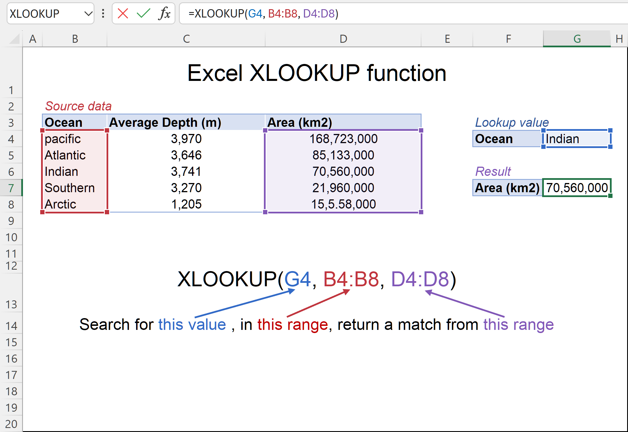
Supposing, you have a summary table with information about the five oceans on the Earth. You want to get the area of a specific ocean input in F1 (lookup_value). With the ocean names in A2:A6 (lookup_array) and areas in C2:C6 (return_array), the formula goes as follows:
=XLOOKUP(F1, A2:A6, C2:C6)
Translated into plain English, it says: search for the F1 value in A2:A6 and return a value from C2:C6 in the same row. No column index numbers, no sorting, no other ridiculous quirks of Vlookup! It just works :)
XLOOKUP availability
As of now, the XLOOKUP function is available in Excel 365, Excel 2021, and Excel for the web. It's important to note that XLOOKUP is not backward compatible, meaning it won't function in earlier versions.
How is XLOOKUP better than VLOOKUP?
XLOOKUP is a powerful function that surpasses VLOOKUP in many aspects. It offers more capabilities, versatility and efficiency. Here are the top 10 features that make it the ultimate lookup function in Excel:
- Vertical and horizontal lookup. The XLOOKUP function got its name due to its ability to look up both vertically and horizontally.
- Look in any direction: right, left, bottom or up. While VLOOKUP can only search in the leftmost column and HLOOKUP in the topmost row, XLOOKUP has no such limitations. The notorious left lookup in Excel is not a pain anymore!
- Exact match by default. In most situations, you will be looking for an exact match, and XLOOKUP returns it by default (unlike the VLOOKUP function that defaults to approximate match). Of course, you can get XLOOKUP to perform an approximate match too if needed.
- Partial match with wildcards. When you know only some part of the lookup value, not all of it, a wildcard match comes in handy.
- Search in reverse order. Earlier, to get the last occurrence, you had to reverse the order of your source data. Now, you simply set the search_mode argument to -1 to force your Xlookup formula to search from the back and return the last match.
- Return multiple values. By manipulating with the return_array argument, you can pull an entire row or column of data related to your lookup value.
- Search with multiple criteria. Excel XLOOKUP handles arrays natively, which makes it possible to perform lookup with multiple criteria.
- If error functionality. Traditionally, we use the IFNA function to trap #N/A errors. XLOOKUP incorporates this functionality in the if_not_found argument allowing to output your own text if no valid match is found.
- Column insertions/deletions. One of the most irritating issues with VLOOKUP is that adding or removing columns breaks a formula because the return column is identified by its index number. With XLOOKUP, you supply the return range, not number, meaning you can insert and remove as many columns as you need without breaking anything.
- Better performance. VLOOKUP could slow down your worksheets because it includes the entire table in calculations, which results in processing far more cells than actually needed. XLOOKUP handles only the lookup and return arrays that it truly depends on.
For more information, please see Difference between VLOOKUP and XLOOKUP.
How to use XLOOKUP in Excel - formula examples
The following examples demonstrate the most useful XLOOKUP features in action. Additionally, you will discover a couple non-trivial uses that will take your Excel lookup skills to a new level.
Look up vertically and horizontally
Microsoft Excel used to have two functions for different lookup types, each having its own syntax and usage rules: VLOOKUP to look vertically in a column and HLOOKUP to look horizontally in a row.
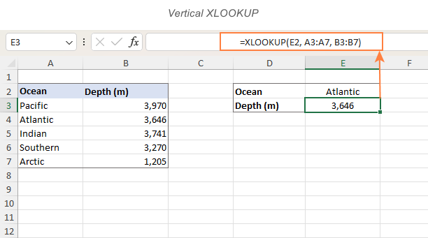
The XLOOKUP function can do both with the same syntax. The difference is in what you provide for the lookup and return arrays.
For v-lookup, supply columns:
=XLOOKUP(E2, A3:A7, B3:B7)
For h-lookup, enter rows instead of columns:
=XLOOKUP(I1, B1:F1, B2:F2)

Left lookup performed natively
In earlier versions of Excel, INDEX MATCH formula was the only reliable way to look to the left or above. Now, you no longer need to combine two functions where one would suffice. Just specify the target lookup array, and XLOOKUP will handle it without a problem regardless of its location.
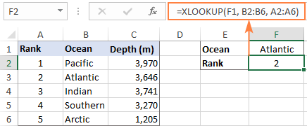
As an example, let's add the Rank column to the left of our sample table. The goal is to get the rank of the ocean input in F1. VLOOKUP would stumble here because it can only return a value from a column to the right of the lookup column. An Xlookup formula copes with ease:
=XLOOKUP(F1, B2:B6, A2:A6)
In a similar manner, you can look above when searching horizontally in rows.
XLOOKUP with exact and approximate match
The match behavior is controlled by the 5th argument called match_mode. By default, an exact match is performed.
Please pay attention that even when you choose an approximate match (match_mode set to 1 or -1), the function will still search for an exact match first. The difference is in what it returns if an exact lookup value is not found.
Match_mode argument:
- 0 or omitted - exact match; if not found - #N/A error.
- -1 - exact match; if not found - next smaller item.
- 1 - exact match; if not found - next larger item.
Exact match XLOOKUP
This is the option you probably use 99% of the time you do lookup in Excel. Since an exact match is XLOOKUP's default behavior, you can omit match_mode and supply only the first 3 required arguments.
In some situations, however, an exact match won't work. A typical scenario is when your lookup table does not contain all the values, but rather "milestones" or "bounds" like quantity-based discounts, sales-based commissions, etc.
Our sample lookup table shows the correlation between exam scores and grades. As you can see in the screenshot below, an exact match works only when the score of a particular student matches the value in the lookup table exactly (like Christian in row 3). In all other cases, an #N/A error is returned.
=XLOOKUP(F2, $B$2:$B$6, $C$2:$C$6)
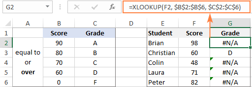
To get the grades instead of #N/A errors, we need to look for an approximate match as shown in the next example.
Approximate match XLOOKUP
To perform an approximate lookup, set the match_mode argument to either -1 or 1, depending on how your data is organized.
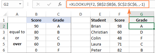
In our case, the lookup table lists the lower bounds of the grades. So, we set match_mode to -1 to search for the next smaller value when an exact match is not found:
=XLOOKUP(F11, $B$11:$B$15, $C$11:$C$15, ,-1)
For example, Brian has the score of 98 (F2). The formula searches for this lookup value in B2:B6 but cannot find it. Then, it searches for the next smaller item and finds 90, which corresponds to grade A:
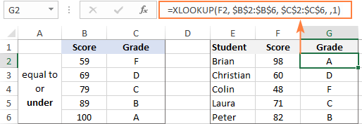
If our lookup table contained the upper bounds of the grades, we would set match_mode to 1 to search for the next larger item if an exact match fails:
=XLOOKUP(F2, $B$2:$B$6, $C$2:$C$6, ,1)
The formula searches for 98 and again cannot find it. This time, it tries to find the next larger value and gets 100, corresponding to grade A:
Tip. When copying an Xlookup formula to multiple cells, lock the lookup or return ranges with absolute cell references (like $B$2:$B$6) to prevent them from changing.
XLOOKUP with partial match (wildcards)
To perform a partial match lookup, set the match_mode argument to 2, which instructs the XLOOKUP function to process the wildcard characters:
- An asterisk (*) - represents any sequence of characters.
- A question mark (?) - represents any single character.
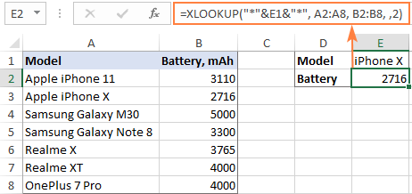
To see how it works, please consider the following example. In column A, you have a few smartphone models and, in column B, their battery capacity. You are curious about the battery of a certain smartphone. The problem is that you are not sure you can type the model name exactly as it appears in column A. To overcome this, enter the part that is definitely there and replace the remaining characters with wildcards.
For example, to get information about the battery of iPhone X, use this formula:
=XLOOKUP("*iphone X*", A2:A8, B2:B8, ,2)
Or, input the known part of the lookup value in some cell and concatenate the cell reference with the wildcard characters:
=XLOOKUP("*"&E1&"*", A2:A8, B2:B8, ,2)
XLOOKUP in reverse order to get last occurrence
In case your table contains several occurrences of the lookup value, you may sometimes need to return the last match. To have it done, configure your Xlookup formula to search in reverse order.
The direction of search is controlled be the 6th argument named search_mode:
- 1 or omitted (default) - searches from first to last value, i.e. top-to-bottom with vertical lookup or left-to-right with horizontal lookup.
- -1 - searches in reverse order from last to first value.
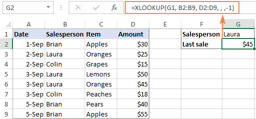
As an example, let's return the last sale made by a specific salesperson. For this, we put together the first three required arguments (G1 for lookup_value, B2:B9 for lookup_array, and D2:D9 for return_array) and put -1 in the 5th argument:
=XLOOKUP(G1, B2:B9, D2:D9, , ,-1)
Straightforward and easy, isn't it?
XLOOKUP to return multiple columns or rows
One more amazing feature of XLOOKUP is its ability to return more than one value relating to the same match. All is done with the standard syntax and without any extra manipulations!
From the below table, supposing you want to retrieve all the details pertaining to the salesperson in F2. What you need to do is supply a range containing several columns (B2:D7) for the return_array argument:
=XLOOKUP(F2, A2:A7, B2:D7)
You enter the formula in the top-left cell of the results range, and Excel automatically spills the results into adjacent blank cells. In our case, the returned array (G2:I2) consists of 1 row and 3 columns (Date, Item and Amount). Looking from another angle, we can say that XLOOKUP returns an entire row of data relating to the lookup value.

If you prefer to arrange the results vertically in a column, nest XLOOKUP into the TRANSPOSE function to flip the returned array:
=TRANSPOSE(XLOOKUP(G1, A2:A7, B2:D7))
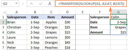
To return values from non-adjacent columns, nest the FILTER function in the return_array of XLOOKUP. A horizontal array {1,0,1} served to the include argument of FILTER determines which columns to filter out (0s) and which to return (1s).
=XLOOKUP(F2, A2:A7, FILTER(B2:D7, {1,0,1}))

It should be noted, however, that XLOOKUP cannot return multiple columns when the lookup_value argument is a range. In this case, you can use the combination of the CHOOSEROWS and XMATCH functions:
=CHOOSEROWS(B2:C10, XMATCH(E2:E4, A2:A10))

Similarly, you can return values from multiple rows when performing a horizontal lookup. To put it differently, you can return an entire column of data relating to your lookup value.
For example, to return all the values from the Amount column, use "Amount" (F1) as lookup_value, the range A1:D1 containing the column headers as lookup_array, and the range A2:D7 as return_array.
=XLOOKUP(F1, A1:D1, A2:D7)
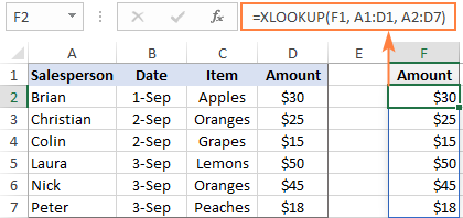
It’s important to ensure that you have enough blank cells to the right or down when using XLOOKUP to return multiple values, as a #SPILL! error will occur if there are not enough empty cells.
Note. If your lookup array contains multiple occurrences of the lookup value and you aim to return all matches, XLOOKUP cannot do that. In this case, you can use the FILTER function or the combination of INDEX, SMALL and ROW functions as demonstrated in this tutorial: How to Vlookup multiple matches in Excel.
Tip. XLOOKUP can also be used to search for and replace values with other values that you specify. A example of such bulk replace can be found here: How to search and replace multiple values with XLOOKUP.
XLOOKUP with multiple criteria
Another big advantage of XLOOKUP is that it handles arrays natively. Due to this ability, you can evaluate multiple criteria directly in the lookup_array argument:
How this formula works: The result of each criteria test is an array of TRUE and FALSE values. The multiplication of the arrays converts TRUE and FALSE into 1 and 0, respectively, and produces the final lookup array. As you know, multiplying by 0 always gives zero, so in the lookup array, only the items that meet all the criteria are represented by 1. And because our lookup value is "1", Excel takes the first "1" in lookup_array (first match) and returns the value from return_array in the same position.
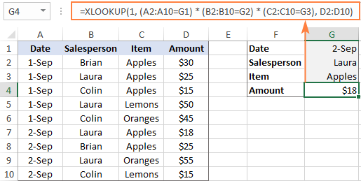
To see the formula in action, let's pull an amount from D2:D10 (return_array) with the following conditions:
- Criteria1 (date) = G1
- Criteria2 (salesperson) = G2
- Criteria3 (item) = G3
With dates in A2:A10 (criteria_range1), salesperson names in B2:B10 (criteria_range2) and items in C2:C10 (criteria_range3), the formula takes this shape:
=XLOOKUP(1, (B2:B10=G1) * (A2:A10=G2) * (C2:C10=G3), D2:D10)
Though the Excel XLOOKUP function processes arrays, it works as a regular formula and is completed with a usual Enter keystroke.
The XLOOKUP formula with multiple criteria is not limited to "equal to" conditions. You are free to use other logical operators as well. For example, to filter orders made on the date in G1 or earlier, put "<=G1" in the first criterion:
=XLOOKUP(1, (A2:A10<=G1) * (B2:B10=G2) * (C2:C10=G3), D2:D10)
For more examples, please see How to use XLOOKUP multiple criteria.
Double / nested XLOOKUP
To find a value at the intersection of a certain row and column, perform the so-called double lookup or matrix lookup. Yep, Excel XLOOKUP can do that too! You simply nest one function inside another:
How this formula works: The formula is based on XLOOKUP's ability to return an entire row or column. The inner function searches for its lookup value and returns a column or row of related data. That array goes to the outer function as the return_array.
For this example, we are going to find the sales made by a particular salesperson within a certain quarter. For this, we enter the lookup values in H1 (salesperson name) and H2 (quarter), and do a two-way Xlookup with the following formula:
=XLOOKUP(H1, A2:A6, XLOOKUP(H2, B1:E1, B2:E6))
Or the other way round:
=XLOOKUP(H2, B1:E1, XLOOKUP(H1, A2:A6, B2:E6))
Where A2:A6 are the salesperson names, B1:E1 are quarters (column headers), and B2:E6 are data values.

A two-way lookup can also be performed with an INDEX Match formula and in a few other ways. For more information, please see Two-way lookup in Excel.
If Error XLOOKUP
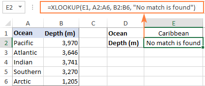
When the lookup value is not found, Excel XLOOKUP returns an #N/A error. Quite familiar and understandable to expert users, it might be rather confusing for novices. To replace the standard error notation with a user-friendly message, type your own text into the 4th argument named if_not_found.
Back to the very first example discussed in this tutorial. If someone inputs an invalid ocean name in E1, the following formula will explicitly tell them that "No match is found":
=XLOOKUP(E1, A2:A6, B2:B6, "No match is found")
Notes:
- The if_not_found argument traps only #N/A errors, not all errors.
- #N/A errors can also be handled with IFNA and VLOOKUP, but the syntax is a bit more complex and a formula is lengthier.
Case-sensitive XLOOKUP
By default, the XLOOKUP function treats lowercase and uppercase letters as the same characters. To make it case-sensitive, use the EXACT function for the lookup_array argument:
How this formula works: The EXACT function compares the lookup value against each value in lookup array and returns TRUE if they are exactly the same including the letter case, FALSE otherwise. This array of logical values goes to the lookup_array argument of XLOOKUP. As the result, XLOOKUP searches for the TRUE value in the above array and returns a match from the return array.
For example, to get the price from B2:B7 (return_array) for the item in E1 (lookup_value), the formula in E2 is:
=XLOOKUP(TRUE, EXACT(E1, A2:A7), B2:B7, "Not found")
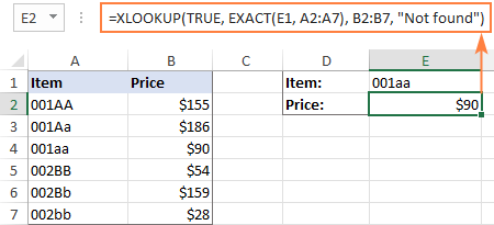
Note. If there are two or more exactly the same values in the lookup array (including the letter case), the first found match is returned.
Excel XLOOKUP not working
If your formula does not work right or results in error, most likely it's because of the following reasons:
XLOOKUP is not available in my Excel
The XLOOKUP function is not backward compatible. It's only available in Excel for Microsoft 365 and Excel 2021, and won't appear in earlier versions.
XLOOKUP returns wrong result
If your obviously correct Xlookup formula returns a wrong value, chances are that the lookup or return range "shifted" when the formula was copied down or across. To prevent this from happening, be sure to always lock both ranges with absolute cell references (like $A$2:$A$10).
XLOOKUP returns #N/A error
An #N/A error just means the lookup value is not found. To fix this, try searching for approximate match or inform your users that no match is found.
XLOOKUP returns #VALUE error
A #VALUE! error occurs if the lookup and return arrays have incompatible dimensions. For instance, it is not possible to search in a horizontal array and return values from a vertical array.
XLOOKUP returns #REF error
A #REF! error is thrown when looking up between two different workbooks, one of which is closed. To fix the error, simply open both files.
As you have just seen, XLOOKUP has many awesome features that make it THE function for almost any lookup in Excel. I thank you for reading and hope to see you on our blog next week!
Practice workbook for download
Excel XLOOKUP formula examples (.xlsx file)
 by
by
139 comments
Perfect Thanks
Hi
how to update xlookup formula in office 2019
Hello,
I am asking XLOOKUP to do a lookup only I get the #NAME?. I honestly can't see what is wrong with my formula.
=XLOOKUP(K:K,'GPS-Data'!A:A,'GPS-Data'!B:B)
Hi! This #NAME? error means that there is no such function in your Excel. See the function description at the beginning of this article.
Hello. This is so useful, thank you.
Is there a way of getting the XLOOKUP to look at and return a value from a different range if the range it is looking at is empty? For example, I am asking it to return a value from B4:T4, by looking up K61 in B12:T12. If B12:T12 is empty, i'd like it to look and to return a value from B9:T9 instead. Is this possible?
My main formula is =XLOOKUP(K61,B12:T12,B4:T4,"") and to solve my problem I have tried =IF(XLOOKUP(K61,B12:T12,B4:T4)="",XLOOKUP(K61,:B9:T9,B4:T4)) but it keeps returning NA when there is definitely a value in B9:T9. Any help greatly appreciated. Thanks
Hello! The following tutorial should help: IF VLOOKUP in Excel: Vlookup formula with If condition. You can do the same with the XLOOKUP function. For example,
=IF(ISNA(XLOOKUP(K61,B12:T12,B4:T4)), XLOOKUP(K61,B9:T9,B4:T4), XLOOKUP(K61,B12:T12,B4:T4))
I hope it’ll be helpful.
Hi,
=XLOOKUP("*B1*",Ordering!L:L,Ordering!A:A, "", 2)
How would I adjust that formula so that the search key(from a drop down menu in B1) returns partial matches eg. JER / TK. from the search range?
Hi! To find a partial match in text values, use these guidelines: How to find substring in Excel. For example:
=XLOOKUP(TRUE,ISNUMBER(SEARCH("B1",Ordering!L:L,Ordering!A:A)), "", 2)
Thank you very much Svetlana for posting the example workbook for practice,
I have been greatly assisted to easily extract interval data from a huge dataset after following your tutorial.
Great thanks indeed🍕👌
Hi! I am trying to create a formula using XLOOKUP that can generate a column average and also work with different quantities of columns (this formula will address survey responses, so, one worksheet may have 10 columns that need to be "looked up", and one may have three). Is there a formula that you would recommend?
Thanks,
Caroline
Hi! The XLOOKUP formula cannot generate any value. It can only find an existing value based on the criteria. To calculate the average value, use these guidelines: How to calculate average in Excel: formula examples, Excel AVERAGEIF function to average cells with condition
Hi
I try to use average with xlookup multiple criteria.
I used Boolean logic to find the first occurrence. and then required average of the previous 60 rows.
than, I used address and cell function to convert values to cell address. than i understand that the outcome is a string so I applied indirect in order to convert to a cell reference an average function can use. unluckily for me the indirect gave value instead of cell address.
it looks something like this:
AVERAGE(INDIRECT(ADDRESS(CELL("row",XLOOKUP(1,(($A:$A>(N300+1/4))*($A:$A1)+(H:H>1)),$B:$B,"-",1,1))-60,CELL("col",XLOOKUP(1,(($A:$A>(N300+1/4))*($A:$A1)+(H:H>1)),$B:$B,"-",1,1)),4,1,))&":"&ADDRESS(CELL("row",XLOOKUP(1,(($A:$A>(N300+1/4))*($A:$A1)+(H:H>1)),$B:$B,"-",1,1)),CELL("col",XLOOKUP(1,(($A:$A>(N300+1/4))*($A:$A1)+(H:H>1)),$B:$B,"-",1,1))))+AVERAGE(INDIRECT(ADDRESS(CELL("row",XLOOKUP(1,(($A:$A>(N300+1/4))*($A:$A1)+(H:H>1)),$B:$B,"-",1,1))-60,CELL("col",XLOOKUP(1,(($A:$A>(N300+1/4))*($A:$A1)+(H:H>1)),$B:$B,"-",1,1)),4,1,)&":"&ADDRESS(CELL("row",XLOOKUP(1,(($A:$A>(N300+1/4))*($A:$A1)+(H:H>1)),$B:$B,"-",1,1)),CELL("col",XLOOKUP(1,(($A:$A>(N300+1/4))*($A:$A1)+(H:H>1)),$B:$B,"-",1,1)))))
any help will be very much appreciated
Hi! It is very difficult to understand a formula that contains unique references to your workbook worksheets. Please clarify your specific problem or provide additional information to understand what you need.
hi Alexander
thanks for your quick response
I'll do my best trying to describe my woorkbook
column A - minutes from 04/01/2022 00:00 until now range from 3 to 650002
column B - Mwt by minute based on column A range from 3 to 650002
column G - is DNI by minute based on column A range from 3 to 650002
column H - is DNI by minute based on column A range from 3 to 650002
column N - Dates by day from 04/01/2022 00:00 until now range from 3 to 452
I would like to get an output as follows: by giving date (column N) find the first time DNI by columns G&H is bigger than 1 and do average by column B and last 60 minutes from first event.
in my previous post you to averages because i need to same output from column D
hope hearing form you soon
Hype
Hi! Here is an example of a formula that might be helpful. The MATCH function finds a position number in the range where the date = N1 and the value in column H is greater than 1 (for example, we get a position number 13). Add 2 to this position number to get the row number. Use the INDIRECT function to get the address of the cell in column B (for example, B15). The function OFFSET returns the range of values from this cell and 5 rows higher (for example B11:B15). Use the AVERAGE function to calculate the average in this range.
=AVERAGE(OFFSET(INDIRECT("B"&MATCH(1,($N$3:$N$20=N1)*(H3:H20>1),0)+2),0,0,-5,1))
I hope my advice will help you solve your task.
Thank you for this very informative article. I am trying to use xlookup to return the smallest of values in the return range where the lookup value occurs multiple times in the lookup range. It looks like it just returns the first one it finds. Is there a way to use the xlookup function as is, or to nest another formula to control which value is returned?
Example:
=XLOOKUP("A-B-C-D",A:A,B:B)
Tag | Sequence
A-B-C-D | 5
C-D-T-G | 4
G-H-E-H | 2
A-B-C-D | 3
B-T-R-D | 1
"A-B-C-D" occurs twice, but would like to return the smaller of the two value (3), instead of (5) as it currently does, without having to change the sort of the table.
Thank you,
-Andres
Hi!
To search by multiple criteria, use the INDEX MATCH functions. You can learn more about MINIFS function in Excel in this article on our blog.
Try this formula:
=INDEX(B1:B5,MATCH(1,(A1:A5="A-B-C-D") * (B1:B5=MINIFS(B1:B5,A1:A5,"A-B-C-D")),0))
Good day,
I'm usinng a list with 28 data in and using xloopup to look for some values.
=$E$2&"-"&C4 This formula is used in 53 rows in column A and this combine the number in the list and number un column C.
The Xlookup is working fine with the first 103 rows that I search, but after that I get the #N/A error.
My question is how big can the Xlookup array be?
=XLOOKUP(A4,Data2!$A$2:$A$1000,Data2!$G$2:$G$1000)
Hi! The XLOOKUP function has no limitations. Error #N/A means that the data is not found. Possible causes are given in the article above.
Hello,
I was particularly interested in the above section on "XLOOKUP to return multiple columns or rows".
Can you tell me, is the return array limited to adjacent columns (as your example per B2:D7 returns information from columns B, C and D.)?
Or is it possible to return information from a table which has many columns but you only want info from for example B, F, K?
Thanks, Janek
Hello! Extract values from all adjacent columns, for example B:D. To get values from only a few columns, for example from B and D, use the CHOOSECOLS function.
Here is an example of this formula:
=CHOOSECOLS(XLOOKUP(F3, A3:A8, B3:D8),1,3)
For more information, please visit: CHOOSECOLS function in Excel to get columns from array or range.
Thank you, that is almost perfect for what I need, though I think I see that when CHOOSECOLS is used, the XLOOKUP lookup value must be a single cell address and not an array itself.
IN the double formula, do I have to use column and row at a time or i can use column and column or row & row? please help me to figure out this problem
Sorry, I do not fully understand the task.
As it's currently written, it's hard to tell exactly what you're asking.
I am trying to figure out if the content of the cells needs to be text or number. i am comparing data from two speadsheets. the last 4 # of telephone #. I use the =RIGHT(cell location, 4) the result is the last 4 #'s of the 10 digit phone #. THe problem is when I am using the xlookup forumla Keep getting an #VALUE! error, I tried to convert both columns to numbers, but I am still gettin the error.
Hi! Unfortunately, I can't see your data and I don't know what formula you used. The LEFT function always returns text. If you convert those 4 digits to a number, you might lose the leading zeros. Note the paragraph above: XLOOKUP with wildcards. Here is an example formula:
=XLOOKUP("*"&RIGHT(E1,4),C1:C12,A1:A12,,2)
Pay attention to Match_mode: 2 - wildcard character match.
I hope it’ll be helpful.
I am trying to work out this formula =IF(A2>0, "Non Compliance","Compliance") but I want to exclude blank cells. How can I do that?
To add a second condition, use IF OR statement.
If I understand your task correctly, try the following formula:
=IF(OR(A2>0, ISBLANK(A2)), "Non Compliance","Compliance")
For more information, please visit: ISBLANK function in Excel to check if cell is blank
Can a nested Xlookup return a result based on criteria in two different columns? I noticed that the most successful results are when there is one horizontal and one vertical.
Hello!
You can read how to do a 2D search by rows and columns in this article - Excel INDEX MATCH MATCH and other formulas for two-way lookup
Hi Paul,
Sure, it can. Please check the "XLOOKUP with multiple conditions" example in this tutorial.
Hello,
I am wondering if it's possible to have a multiple results but from the same column.
For example I have value X that I am trying to find in column ''Y'' and than return the value from column ''Z'' next to it. This is pretty standard.
But X appears a few times in ''Y'' with different value in ''Z'' - and I want the formula to return all those different values. Is it possible?
Hello!
If I understand your task correctly, the following tutorial should help: How to VLOOKUP multiple values in Excel with criteria. I hope I answered your question.
Hello!
The instruction that you linked is exactly what I need (this section: Vlookup to return multiple results in one cell (comma or otherwise separated)).
My issue is that the values I want returned are on the left side of the cell with the looked up value - that's why I was wondering if it's possible to do something like that with xlookup since here we don't have to worry about that.
Hi!
I don't think you opened the article I recommended. Do that and see that the VLOOKUP function is not used and the order of the columns is irrelevant.
Thanks for the great article. Wondering if you can suggest if it is useful for my situation below:
I am trying to categorize purchases from my credit card bill. The entries look something like this:
A B
MARKS&SPENCER LONDON $100
ITUNES 1234 $0.99
TESCO PAY AT PUMP LIVERPOOL $97.00
MARKS&SPENCER GATESHEAD $15.00
ITUNES 0987 $0.99
Column C should classify each item into a category (eg Supermarket, iTunes or Petrol) based on the content of Column A. I am currently using a IFS(ISNUMBER(SEARCH formula to check column A for partial text (i.e. "MARKS&SPENCER") and return a category but the formula has become very long. Can this be done using an array instead?
Hello!
Use the SEARCH function to determine partial matching of text strings.
=INDEX($E$1:$E$5,MATCH(TRUE,ISNUMBER(SEARCH($E$1:$E$5,A2)),0))
Use INDEX MATCH to get the desired value from the list of categories $E$1:$E$5. I hope it’ll be helpful. If something is still unclear, please feel free to ask.
Thank you Alexander, that got the job done
Cheers
I am using a XLOOKUP in order to sort and match results between two tables based on a unique ID number.
the formula I am using looks like this: =XLOOKUP(A2,LiveProjects!M:M,LiveProjects!P:P,"",0,1)
This seems to be working only for SOME of the IDs i have in the table I am using, but not all. Does this not work if you are searching using a value in A2 which is the result of another formula?
I.e. does the look up only look in the text in the cell and not the result given by that text?
Hello!
The XLOOKUP function works with values that are the result of other formulas. If these values are numbers, pay attention to the decimal values and use round numbers.
How do I get a return of multiple column headers by matching a repeated row value using Xlookup? Ex. Column headers are different shopping centers and rows are different items. I am trying to look up a specific item (row) and the return to be a list of column headers (shopping centers) that sell the item. Thank you
Hi - this is the best tutorial I've come across. Thanks
1- I have two Sheets (LISTING= with columns: Vendor Name, ID# and Hotel; & HOTEL= with 9 columns that contain the first 3 cols as: Priority Vendor1, ID# & Email ; Priority Vendor2, ID# & Email; and Priority Vendor3, ID# & Email
2- I need to return the vendor name found on either one of the Priority Vendor1, 2 or 3 cols based on the ID# on the LISTING sheet, but I haven't been able to get results by doing a search of the ID# on (sheet1) on the 3 cols of sheet2
Is this possible?
Hello!
Each of your three columns is a separate table for the VLOOKUP or XLOOKUP functions. Try this guide with examples: How to VLOOKUP across multiple sheets in Excel.
I hope it’ll be helpful. If something is still unclear, please feel free to ask.
I am comparing 2 columns. The first column has 16318 rows and the second 18526 rows. The formula =XLOOKUP(C2, B2:B18584, A2:A18584, "No match is found") works perfectly.
My question: Is there a way to populate the formula in column "D" incrementing the C2 value without changing the range values? When I use ctl and pull the corner of the cell down to copy into subsequent cells the first cell value of the ranges also increments resulting the elimination of one cell for every copy.
Example: =XLOOKUP(C61, B61:B18584, A61:A18584, "No match is found")
Thanks for your insight.
Hello!
To keep cell references unchanged when you copy a formula, use absolute cell references. Please have a look at this article: Why use dollar sign ($) in Excel formulas - absolute and relative cell references.
Alright I know this is very late but I must let you know how much I appreciate this response. It has corrected something that was plaguing me tremendously and saved so much data entry time. Thank you for the assist.
Is XLookup able to return the first result that has a negative number?
Hello!
To search by condition, use INDEX MATCH.
=INDEX(A1:A10,MATCH(TRUE,A1:A10<0,0))
Hope this is what you need.
Is there a way to use xlookup (or maybe it would be something else) to return one value from two. To explain I have a table in document 1 that has included in it first names (column c) and last names (column B) and I want it to find and input the ID number (column A) from document 2. Document 2 has all of the above information and other information that I don't need, all in separate columns. So I need it to get a match to both first and last name for it to get the ID number. Unfortunately, the way it is set up, I cannot do the inverse and input the ID numbers and search for the first and last names. Is there a way to do this? Another option is I can have it in document 1 as LastName, First Name in column B and ID number in column A, but document 2 would still have the last name and first name separate.
Thanks in advance!!
Hello!
You can search by two criteria with INDEX+MATCH or XLOOKUP. See formula examples here.
To input the ID numbers and search for the first and last names, you can use the paragraph in this article above: XLOOKUP to return multiple columns or rows.
I hope I answered your question. If something is still unclear, please feel free to ask.
I'm trying build out an excel file using two sheets. I'm trying to use the ID# from column A sheet one to find said ID# from sheet two. Then I'd like it to search for the row title from sheet 1 on sheet 2 to pull sheets 2s value into sheet 1. Is this possible?
Hello!
If I understand your task correctly, pay attention to the following paragraph of the article above: Double XLOOKUP.
To correctly write a reference to another sheet in a formula, use these examples: Excel reference to another sheet or workbook (external reference).
Hope this is what you need.
How would you use the function of xlookup in excel? And what was the function names before as?
Someone can answer this please. Thanks in advance ?
Hi! I'm trying to use XLOOKUP for the following situation but I don't know how to do so the number of cals finds the right pricing tier.
I have 1 table with 14 columns: a) a CONCAT formula to add in 1column the centre, market & channel info (BsAsARGcall) b) different pricing tiers, under 4000 calls there's a price for each centre, market & channel and the same for every tier: over 8000, over 10000 calls, etc there's a different price according to amount of contacts
In another table I have a column with another CONCAT formula same info as above (centre, market,channel) and then the column with amount of calls per centre, market, channel.
What I need to do is for the XLOOKUP to find the right price by searching the right tier column (under 4000, over 8000, etc) and bring the right price according to the amount of calls. Any help? Hope I was able to explain myself clearly :-)
Hi,
I need to retrieve data under certain conditions from one sheet to another, and here is the formula I am using: =XLOOKUP((IF(OR('by sample'!$H4="cheek, right",'by sample'!$H4="cheek, left"),'by sample'!$H4,"")),'by sample'!$H4:$H1000,'by sample'!B4:B1000,,0).
It works well, but when the results is N/A I would like excel to find the next xlookup value.
I am trying to write an IFNA of the sort: IFNA(XLOOKUP(...), find next xlookup value) to avoid removing the cells manually/with find and select tool, but without success...
How could I proceed?
Hi!
I recommend reading this guide: How to use IFNA function in Excel with examples. This should solve your task.
HI,
I am trying to copy down the XLOOKUP function to use it for an entire column but it is changing the search array.
EXP.
XLOOKUP(B1, C2:C6, D3:D7) then when I copy down I want XLOOKUP(B2, C2:C6, D3:D7) but I get XLOOKUP(B2, C3:C7, D4:D8). It shifts all by 1 cell instead of just the search value.
How do I get it to automatically shift the search but not the other 2 array?
Thanks
Hello!
Use absolute references in the formula. I recommend this article: Why use dollar sign ($) in Excel formulas - absolute and relative cell references.
This should solve your task.
Hello - has this replaced the use of Transpose and Filter? I used to use this formula to look up an array that had multiple instances and returns in one column: "=TRANSPOSE(FILTER(C2:C6, B9=B2:B6))". Where C2:C6 had the expected outputs (more than one output but only in one column) B9 is the criteria to lookup and B2;B6 is the array to look for it in.
When I use it now I need a NAME error which seems to indicate its no longer a recognized formula name.
I cant find the equivalent in the xlookup formula i.e. where the multiple responses are all in the same column.
Hi!
The NAME error means that your version of EXCEL does not contain the function you want to use.
Please have a look at this article - How to VLOOKUP multiple values in Excel with criteria.
Very informative, thank you. I was particularly interested in XLOOKUP with multiple criteria. You use:
XLOOKUP(1, (criteria_range1=criteria1) * (criteria_range2=criteria2) , return_array)
I had not seen this before, and previously I had used concatenation, for example:
XLOOKUP(criteria1 & criteria2, criteria_range1 & criteria_range2, return_array)
But this can be very slow if you are referencing whole columns. Do you know if your approach is faster? I suspect it would be.
Hello!
I do not recommend using the entire column as criteria_range (for example, A:A). This will slow down the calculations significantly. Use the range where the data is actually located (for example, A2:A100).
Thanks Alexander. Yes I appreciate that using specific ranges is faster than entire columns. In some models though I find column references are preferable, as the formulas are easier to read and you don't have to worry about users adding new data to rows outside the range.
I guess my question is, *for a given range of data*, whether there is a significant difference in speed between the two XLOOKUP approaches above. I might have a play around to see.
Hi -
this may not be an xlookup question.
I have one sheet with a list of protein names in column A, and on another sheet, a list of biological pathways (column A), with the corresponding proteins that are found in that pathway listed across columns B-Z in that row. Every pathway has column B filled (at least 1 protein per pathway), but after that has a variable number of entries depending on how many proteins are associated with that pathway (from 1 up to 25, with any remaining cells blank). All proteins on sheet 2 are contained in the list on sheet 1, and vice versa. There should be no "not founds".
I want to enter a formula in sheet 1 by which sheet 2 will be searched for each protein name and for each, return which pathways it is associated with, returning those pathway names into sheet 1, column B (and C and D and so on until all relevant pathways are listed).
a small made up example, separate column entries separated by pipes
sheet 1 (single letter protein names)
A
B
C
D
sheet 2 (pathway name|protein|protein|protein)
Notch|A|B|C|D
WNT|A|B|D
EGFR|C|D|A
RAS|D
desired results, sheet 1:
A|Notch|WNT|EGFR
B|Notch|WNT
C|Notch|EGFR
D|Notch|WNT|EGFR|RAS
Any help appreciated.
thanks
Hello!
To get data by condition, you can use the FILTER function.
I believe the following formula will help you solve your task:
=TRANSPOSE(INDEX(FILTER(Sheet2!$A$1:$E$4,(Sheet2!$B$1:$B$4=Sheet1!A1)+(Sheet2!$C$1:$C$4=Sheet1!A1)+(Sheet2!$D$1:$D$4=Sheet1!A1)+(Sheet2!$E$1:$E$4=Sheet1!A1)),,1))
Do you know what is the correct syntax if I would like to implement the following query inside of a VBA code? =XLOOKUP(1, (B2:B10=G1) * (A2:A10=G2) * (C2:C10=G3), D2:D10)
I would like to implement the following, which works well in pasted in a cell:
=XLOOKUP(1;(Elisa!$J$2:$J$2015=BH$2)*(Elisa!$B$2:$B$2015=$AY7);Elisa!$E$2:$E$2015;" ")
What I have tried:
Worksheets("Adatbázis").Cells(H, I).Value = WorksheetFunction.XLookup(1, (Worksheets("Elisa").Range("J2:J2015") = Cells(2, I)) * (Worksheets("Elisa").Range("B2:B2015") = Cells(H, 51)), Worksheets("Elisa").Range("E2:E2015"), " ")
This always ends with a Tyme mismatch message around this part: Worksheets("Elisa").Range("J2:J2015") = Cells(2, I). I have tried it several ways but no luck so far...
Hello!
Unfortunately, we cannot help you with VBA.
I really like the xlookup function but I am struggling with a situation I am unable to resolve.
I want to use the xlookup to find a transaction in a check register and put that transaction in a budget report. I am able to get xlookup to find a single line item for a budget category but when a category has multiple entries xlookup is only returning the first line item of that category. What I am after is not only to find the first transaction of a particular category but to find all of them and add(sum) them all together into one cell. ex: find all amounts paid for groceries then sum them all together.
I am using the date & category as a reference to find the amount paid in each category. Here is the formula I am using it only finds the first transaction. How do I need to change it to find all transactions and sum them all together in one cell?
=IFERROR(XLOOKUP($J$4&F15,'Arvest Savings'!$C:$C&'Arvest Savings'!$E:$E,'Arvest Savings'!$H:$H,,0),"")
The above formula is going into the budget form under the actual column then once the entry is made in the check register it automatically populates into the budget form for the appropriate month,
It works great for a single transaction where I need assistance is with finding multiple transactions and getting them summed all together.
Hello!
To conditionally sum values, you can use the SUMIFS function. Here is a guide with examples: Excel SUMIFS and SUMIF with multiple criteria.
I hope my advice will help you solve your task.
how does xlookup work for multiple tables - two similar sets of data, one for onshore and one for offshore. I have Line of work (Java, testing etc), Designation (Manager, Team lead, etc), rate for line of work vs designation. This calculation is straight forward if its only for offshore or onshore. Now If i have to get both in one formula should I use IFERROR ?
Hello!
I recommend reading this guide: How to VLOOKUP across multiple sheets in Excel. You can use all these instructions with the XLOOKUP function.
I'm struggling with XLOOKUP and dates with multiple criteria. Please help!
I'm trying to return a Lab value for a particular ID collected on a date that is closest to, but before or equal to, the Clinic Date.
For example for ID: A251527 on Clinic Date 17/09/2008 (in cells E2 and F2 respectively).
The answer should be 130 on 12/08/2008 but XLOOKUP using multiple criteria seems to return the Lab value on the first date for this ID (124).
=XLOOKUP(1, ($A$2:$A$17="ID")*(LARGE($B$2:$B$17,COUNTIF($B$2:$B$17,">"&$F$2)+1)<=F2), $C$2:$C$17)
The data is unsorted and is large ~110,000 rows.
Clean ID Date Collected Lab value ID Clinic date
A251300 17/09/2008 118 A251527 17/09/2008
A251300 16/09/2008 129
A251527 13/06/2008 124
A251527 16/06/2008 115
A251527 18/06/2008 114
A251527 23/06/2008 113
A251527 24/06/2008 108
A251527 24/06/2008 113
A251527 12/08/2008 130
A251527 03/11/2008 133
A251527 19/02/2009 120
A251527 20/02/2009 112
A251527 21/02/2009 122
A251527 22/02/2009 138
A252601 19/08/2008 136
A252601 10/02/2009 117
Hello!
You cannot apply XLOOKUP approximate search on unsorted data.
If I got you right, the formula below will help you with your task:
=INDEX(C2:C17,MATCH(MAX(IFERROR((B2:B17-E2) / ((A2:A17=D2)*((B2:B17-E2)<0)),-100000)), (A2:A17=D2)*(B2:B17-E2),0))
In Excel 365:
=VLOOKUP(E2,SORT(FILTER(B2:C17,(B2:B17 < E2)*(A2:A17=D2)),2,1),2,1)
I hope my advice will help you solve your task.
Thanks for replying.
Your VLOOKUP formula for Excel 365 seems to be missing some arguments at the end? Can you complete please?
hi
thank you for the post, very useful
how can I set the Xlookup function to get the first, second, and third result on arranged set when working with multiple data in a table
Hello!
I recommend reading this guide: Vlookup and return nth match.
In these examples, you can use XLOOKUP instead of the VLOOKUP function.
thank you for your prompt answer
greetings!
Hi,
i'm trying to find out Balance Work = Scope of work - Work Done, but result always wrong.
Please help, how to i get final result with XLOOKUP or any other function.
Below given data is Length (m) (From-To).
Scope of work - Work Done = Balance Work
From To From To
62000 66000 68000 68480
67200 71080 68680 69300
72000 73400 73000 73180
73650 75500 76300 76600
76300 76600
77400 78080
78300 79100
79300 79600
Hi!
I don't really understand what you want to calculate. Why are 4 columns used? Describe in more detail. Specify the expected result.
This data is related to Highway construction. in which digit shows location of highway. Terms used means:
1. Scope of work = Construction work to be execute at that locations. (A)
2. Work Done = Construction work has been done. (B)
3. Balance Work = Remaining work, which is to be execute within scope of work. (C=A-B) (Result)
4. From = Starting Point of work (62+000)
5. To = Ending Point of work (66+000)
(From) 62+000 - (To) 66+000 = 4000 m (Length)
Example:
Scope of work (A) Work Done (B) Balance Work (A-B) (Result)
From To Length From To Length From To Length
62+000 66+000 4000 62+000 66+000 4000 68+085 69+630 1545
67+200 71+080 3880 67+200 68+085 885 70+015 70+065 050
72+000 73+400 1400 69+630 70+015 385 72+000 72+100 100
- 70+065 71+080 1015 73+175 73+310 135
- 72+100 73+175 1075
- 73+310 73+400 090
This is highway measurement that's why i used 4 columns.
I have Scope & Work Done Data and i would like to calculate Balance Work.
I hope this will helpful to understand.
Please Help !
Hello!
To find the difference between numbers as text 73+175 and 72+100,
try the formula
=--SUBSTITUTE(B1,"+","")-SUBSTITUTE(A1,"+","")
Hope this is what you need.
HI,
=--SUBSTITUTE(B1,"+","")-SUBSTITUTE(A1,"+","")
Formula suggested by you not solving my problem. May be i am not Letting you know what i want.
Thank you for help !
Hi.
I have a strange issue with XLookup and structured referencing, and I cannot for the life of me work out what I’m doing wrong.
=XLookup(A2,B:B,G:G) works, but =Xlookup(A2,Table1[ColumnB],Table1[ColumnG]) doesn’t - I get a #VALUE ERROR. Column G contains numbers. There are no spaces or other things that usually cause value errors.
I don’t think the problem is with my syntax. The table is named Table1, and the two columns are named as above. I have used xlookup in the same format referencing other tables in the worksheet with no issues.
Any help appreciated.
Hello!
The formula works for me. I was unable to get this error. Check the column names in your table. Column sizes must be the same.
Thanks Alexander. It seems my problem was using a mixture of structured table references and named ranges in the Xlookup formula. This seems not to be allowed.
Hi everyone,
I need to perform XLOOKUP such that the criteria is Difference/Subtraction between two cells of column X and column Y. Suppose Quarter 1,2 as columns and i need to check rows where element/value of Quarter2 - element/value of Quarter1 = 25.
In other words rows in which the difference/subtraction of Column X and Column Y is exactly equal to 25
Hello!
Please try the following formula:
=XLOOKUP(1,--(A2:A10-B2:B10=25),A2:B10)
This formula only returns the first value found. To get all values that meet the criteria, use the FILTER function:
=FILTER(A2:B10,A2:A10-B2:B10=25)
Hope this is what you need.
I need to find and list all possible matches for a 'PART NAME" within a column containing FULL NAMES. Example:
1. JOHN TERRY
2. ADAM JOHN
3. ADAM TERRY
4. CRUISE JOHN
5. JONATHAN JOHN
I need to do an XLOOKUP to list all matching Rows containing "JOHN"
Hello!
XLOOKUP can only return one match, not a list of values. If you need to return a list of values that contain "JOHN", use this tutorial: How to VLOOKUP multiple values in Excel.
=IFERROR(INDEX($A$1:$A$10, SMALL(IF(ISNUMBER(SEARCH($B$1,$A$1:$A$10,1)), ROW($A$1:$A$10)-1,""), ROW()-1)),"")
This array formula is on line 2. Copy it down the column.
I hope I answered your question. If you have any other questions, please don’t hesitate to ask.
Please help how to retrieve the values using vba.
Excel Sheet Name: Source.xlsx (Column: G -> Code)
Excel Sheet Name: Mappings.xlsx (Column: A -> Node; Column: B -> Code)
Example:
In Mappings.xlsx sheet:
When I filter by Code = 001 in Column B, there are 3 rows shown as a result with Column: A values as "001", "00100100", "00100")
So basically one Code has multiple Nodes. I want to retrieve all the Nodes for a specific Code in vba.
I tried with Xlookup, but its retrieving only one value for me and not all the 3 values.
Thanks for your info on XLOOKUP, it was very helpful. Correct my thinking here in case it's wrong, but the XLOOKUP multiple criteria is used to construct an array (column or row) of data but can't return a multi-dimensional array (area) to be searched. Originally I was trying figure out how to use multiple criteria to filter results from a long data table during the XLOOKUP function and wasn't getting anywhere when I realized that I needed to filter the results before I performed the Xlookup. Using the concept of array-based inputs for XLOOKUP, I came up with this ...
=XLOOKUP(0,INDEX(FILTER(A:T,A:A=D3),0,20),INDEX(FILTER(A:T,A:A=D3),0,17))
D3 is the value I want to filter by
A:A is the column I want to filter
A:T are the columns I want FILTER to return to INDEX
0 is the value I want to search for
T (20) is the column I want to search
Q (17) is the column I want to return data from
This allows a custom filter to be applied to the data without modifying the original at all and returns it to the function instead of placing it in a temporary or new cell location. The FILTER functions can also have SORT applied to them before the INDEX for the bitwise searches that require it. Just make sure that what is fed to each INDEX part of the function are identical. I'm posting this here as a search for XLOOKUP combined with FILTER like this doesn't come up in any searches.
Is not working if lookup array & return array from other sheet. Can you help please
Hello!
Please check out the following article on our blog, it’ll be sure to help you with your task: How to Vlookup from another sheet in Excel.
I hope it’ll be helpful.
HI, I have a dataset with staff completing their inspections on specific dates for certain street addresses.
Ex.
Header rows:
1)Area
2) Segment
3)Boundaries
4)Approx. Blocks
5)# Inspectors
6) Bureau
7)Team Lead
8)Completed 12/7
9)Completed 12/8
10)Completed 12/9
11)Completed 12/10
12)Completed 12/11
If I want to get the latest value from #8-#12 columns, what syntax can I use?
Thanks this is great! For some reason the search in reverse order is not working.
Using your example my sheet has (=XLOOKUP(G1,B2:B9,D2:D9, ,-1)) still gives me $25 as the result, not $45.
All the other examples seem to work great
Hi Dave,
Thank you for pointing out this issue!
It looks like Microsoft has changed the order of arguments in the XLOOKUP function! At the moment of writing, this function was a beta available for Office Insiders. That time, search_mode that controls the direction of search was the 5th argument. Now, it's the last (6th) argument. I will review and update all the affected examples ASAP.
In the meantime, please use this formula to get the last occurrence:
=XLOOKUP(G1, B2:B9, D2:D9, , ,-1)
Hi Svetlana,
Very complete but I am stuck with a more complex issue.
I need to get a value based on 3 criteria, including one that is an approximate (i.e. lookup value would be within a range)
My formula looks like this:
=xlookup(Value01&Value02&Value03,Range01&Range02&Range03,ReturnRange,,-1) where value 03 is the approximate crlteria.
The ranges are same lenghts and side by side. It should work however it gives me random return values, never consistent.
Please help.
I have multiple Xlookup's running in my workbook, but I'm having issues with a particular one. I have a column with pay type data (regular time, overtime) and another column where the job name is listed. I am attempting to use xlookup to determine which pay type AND if the job name is one of 3 possibilities (referencing a range of cells for that data) have it return a job type number listed in another range of cells. My current formula is =XLOOKUP($E2,AC2:AC5&($T1,AE2:AE5),AD2:AD5,E2)which returns "regular time" as the answer (which I only want it to do if it won't be replacing the data with information from the proper range). I have to be missing part of the query, but I'm not sure where.
Hello!
I’m sorry but your task is not entirely clear to me. Could you please describe it in more detail?
What do you want to determine using this formula? Pay type? Job type? What is written in cell E2? What is written in cell T1? You are using 3 ranges of AC2: AC5 AE2: AE5 AD2: AD5. What is written in them? Without this, I cannot understand the logic of your formula
Is it possible to utilize an XLOOKUP in conjunction with a range? I'd like to return a value based on a range that varies depending on the lookup criteria.
Example. Criteria one is a customer name, Criteria two is their sales, Result/Return is a order frequency. There is 5 possible return values of what the order frequency should be based on the range of sales and the customer name. There are different ranges based on customer names.
Hello Robert!
Read carefully the section above "XLOOKUP with multiple criteria" You did not explain what you mean by "order frequency".
I’m sorry but your task is not entirely clear to me. For me to be able to help you better, please describe your task in more detail. Please specify what you were trying to find, what formula you used and what problem or error occurred. Give an example of the source data and the expected result.
It’ll help me understand it better and find a solution for you. Thank you.
I couldn't find xlookup in excel 2019
Hi Hamada,
Currently XLOOKUP is only available to users of the Office 365 Insiders channel.
Update: the XLOOKUP function is now available in the Monthly channel of Office 365 subscriptions. Starting in July 2020, it is planned to be included in the Semi-Annual channel.
Hi
I am trying to work out this formula =IF(A2>0,"Non Compliance","Compliance")but i want to exclude blank cells. How do i do that?
thanks
Stephane
Hi Stephane,
You can nest another IF function that checks for blanks, like this:
=IF(A2="","", IF(A2>0,"Non Compliance","Compliance"))