Microsoft Excel provides several functions purposed for counting different kinds of cells, such as blanks or non-blanks, with number, date or text values, containing specific words or character, etc.
In this article, we will focus on the Excel COUNTIF function that is purposed for counting cells with the condition you specify. First, we will briefly cover the syntax and general usage, and then I provide a number of examples and warn about possible quirks when using this function with multiple criteria and specific types of cells.
In essence, COUNTIF formulas are identical in all Excel versions, so you can use the examples from this tutorial in Excel 365, 2021, 2019, 2016, 2013, 2010 and 2007.
COUNTIF function in Excel - syntax and usage
Excel COUNTIF function is used for counting cells within a specified range that meet a certain criterion, or condition.
For example, you can write a COUNTIF formula to find out how many cells in your worksheet contain a number greater than or less than the number you specify. Another typical use of COUNTIF in Excel is for counting cells with a specific word or starting with a particular letter(s).
The syntax of the COUNTIF function is very simple:
As you see, there are only 2 arguments, both of which are required:
- range - defines one or several cells to count. You put the range in a formula like you usually do in Excel, e.g. A1:A20.
- criteria - defines the condition that tells the function which cells to count. It can be a number, text string, cell reference or expression. For instance, you can use the criteria like these: "10", A2, ">=10", "some text".
And here is the simplest example of Excel COUNTIF function. What you see in the image below is the list of the best tennis players for the last 14 years. The formula =COUNTIF(C2:C15,"Roger Federer") counts how many times Roger Federer's name is on the list:
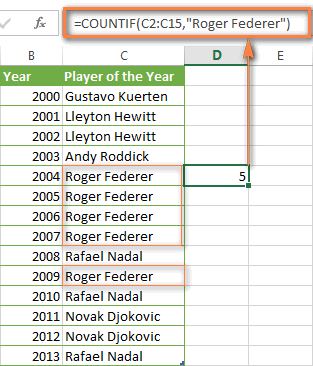
Note. A criterion is case insensitive, meaning that if you type "roger federer" as the criteria in the above formula, this will produce the same result.
Excel COUNTIF function examples
As you have just seen, the syntax of the COUNTIF function is very simple. However, it allows for many possible variations of the criteria, including wildcard characters, the values of other cells, and even other Excel functions. This diversity makes the COUNTIF function really powerful and fit for many tasks, as you will see in the examples that follow.
COUNTIF formula for text and numbers (exact match)
In fact, we discussed the COUNTIF function that counts text values matching a specified criterion exactly a moment ago. Let me remind you that formula for cells containing an exact string of text: =COUNTIF(C2:C15,"Roger Federer"). So, you enter:
- A range as the first parameter;
- A comma as the delimiter;
- A word or several words enclosed in quotes as the criteria.
Instead of typing text, you can use a reference to any cell containing that word or words and get absolutely the same results, e.g. =COUNTIF(C1:C9,C7).
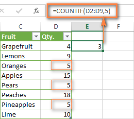
Similarly, COUNTIF formulas work for numbers. As shown in the screenshot below, the below formula perfectly counts cells with quantity 5 in Column D:
=COUNTIF(D2:D9, 5)
In this article, you will find a few more formulas to count cells that contain any text, specific characters or only filtered cells.
COUNTIF formulas with wildcard characters (partial match)
In case your Excel data include several variations of the keyword(s) you want to count, then you can use a wildcard character to count all the cells containing a certain word, phrase or letters as part of the cell's contents.
Suppose, you have a list of tasks assigned to different persons, and you want to know the number of tasks assigned to Danny Brown. Because Danny's name is written in several different ways, we enter "*Brown*" as the search criteria =COUNTIF(D2:D10, "*Brown*").
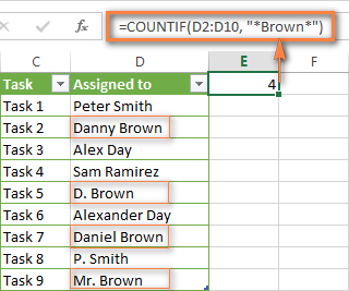
An asterisk (*) is used to find cells with any sequence of leading and trailing characters, as illustrated in the above example. If you need to match any single character, enter a question mark (?) instead, as demonstrated below.
Tip. It is also possible to use wildcards with cell references with the help of the concatenation operator (&). For example, instead of supplying "*Brown*" directly in the formula, you can type it in some cell, say F1, and use the following formula to count cells containing "Brown": =COUNTIF(D2:D10, "*"&F1&"*")
Count cells beginning or ending with certain characters
You can use either wildcard character, asterisk (*) or question mark (?), with the criterion depending on which exactly result you want to achieve.
If you want to know the number of cells that start or end with certain text no matter how many other characters a cell contains, use these formulas:
=COUNTIF(C2:C10,"Mr*") - count cells that begin with "Mr".
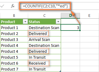
=COUNTIF(C2:C10,"*ed") - count cells that end with the letters "ed".
The image below demonstrates the second formula in action:
If you are looking for a count of cells that start or end with certain letters and contain the exact number of characters, you use the Excel COUNTIF function with the question mark character (?) in the criteria:
=COUNTIF(D2:D9,"??own") - counts the number of cells ending with the letters "own" and having exactly 5 characters in cells D2 through D9, including spaces.
=COUNTIF(D2:D9,"Mr??????") - counts the number of cells starting with the letters "Mr" and having exactly 8 characters in cells D2 through D9, including spaces.
Tip. To find the number of cells containing an actual question mark or asterisk, type a tilde (~) before the ? or * character in the formula. For example, =COUNTIF(D2:D9,"*~?*") will count all cells containing the question mark in the range D2:D9.
Excel COUNTIF for blank and non-blank cells
These formula examples demonstrate how you can use the COUNTIF function in Excel to count the number of empty or non-empty cells in a specified range.
COUNTIF not blank
In some Excel COUNTIF tutorials and other online resources, you may come across formulas for counting non-blank cells in Excel similar to this one:
=COUNTIF(A1:A10,"*")
But the fact is, the above formula counts only cells containing any text values including empty strings, meaning that cells with dates and numbers will be treated as blank cells and not included in the count!
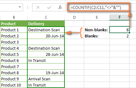
If you need a universal COUNTIF formula for counting all non-blank cells in a specified range, here you go:
Or
This formula works correctly with all value types - text, dates and numbers - as you can see in the screenshot below.
COUNTIF blank
If you want the opposite, i.e. count blank cells in a certain range, you should adhere to the same approach - use a formula with a wildcard character for text values and with the "" criteria to count all empty cells.
Formula to count cells not containing any text:
Since an asterisk (*) matches any sequence of text characters, the formula counts cells not equal to *, i.e. not containing any text in the specified range.
Universal COUNTIF formula for blanks (all value types):
The above formula correctly handles numbers, dates and text values. For example, here's how you can get the number of empty cells in the range C2:C11:
=COUNTIF(C2:C11,"")
Please be aware that Microsoft Excel has another function for counting blank cells, COUNTBLANK. For instance, the following formulas will produce exactly the same results as the COUNTIF formulas you see in the screenshot above:
Count blanks:
=COUNTBLANK(C2:C11)
Count non-blanks:
=ROWS(C2:C11)*COLUMNS(C2:C11)-COUNTBLANK(C2:C11)
Also, please keep in mind that both COUNTIF and COUNTBLANK count cells with empty strings that only look blank. If you do not want to treat such cells as blanks, use "=" for criteria. For example:
=COUNTIF(C2:C11,"=")
For more information about counting blanks and not blanks in Excel, please see:
COUNTIF greater than, less than or equal to
To count cells with values greater than, less than or equal to the number you specify, you simply add a corresponding operator to the criteria, as shown in the table below.
Please pay attention that in COUNTIF formulas, an operator with a number are always enclosed in quotes.
| Criteria | Formula Example | Description |
|---|---|---|
| Count if greater than | =COUNTIF(A2:A10,">5") | Count cells where value is greater than 5. |
| Count if less than | =COUNTIF(A2:A10,"<5") | Count cells with values less than 5. |
| Count if equal to | =COUNTIF(A2:A10,"=5") | Count cells where value is equal to 5. |
| Count if not equal to | =COUNTIF(A2:A10,"<>5") | Count cells where value is not equal to 5. |
| Count if greater than or equal to | =COUNTIF(C2:C8,">=5") | Count cells where value is greater than or equal to 5. |
| Count if less than or equal to | =COUNTIF(C2:C8,"<=5") | Count cells where value is less than or equal to 5. |
You can also use all of the above formulas to count cells based on another cell value, you will just need to replace the number in the criteria with a cell reference.
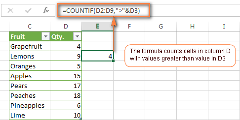
Note. In case of a cell reference, you have to enclose the operator in quotes and add an ampersand (&) before the cell reference. For example, to count cells in the range D2:D9 with values greater than a value in cell D3, you use this formula =COUNTIF(D2:D9,">"&D3):
If you want to count cells that contain an actual operator as part of the cell's contents, i.e. the characters ">", "<" or "=", then use a wildcard character with the operator in the criteria. Such criteria will be treated as a text string rather than a numeric expression. For example, the formula =COUNTIF(D2:D9,"*>5*") will count all cells in the range D2:D9 with contents like this "Delivery >5 days" or ">5 available".
Using Excel COUNTIF function with dates
If you want to count cells with dates that are greater than, less than or equal to the date you specify or date in another cell, you proceed in the already familiar way using formulas similar to the ones we discussed a moment ago. All of the above formulas work for dates as well as for numbers. Let me give you just a few examples:
| Criteria | Formula Example | Description |
|---|---|---|
| Count dates equal to the specified date. | =COUNTIF(B2:B10,"6/1/2014") | Counts the number of cells in the range B2:B10 with the date 1-Jun-2014. |
| Count dates greater than or equal to another date. | =COUNTIF(B2:B10,">=6/1/2014") | Count the number of cells in the range B2:B10 with a date greater than or equal to 6/1/2014. |
| Count dates greater than or equal to a date in another cell, minus x days. | =COUNTIF(B2:B10,">="&B2-"7") | Count the number of cells in the range B2:B10 with a date greater than or equal to the date in B2 minus 7 days. |
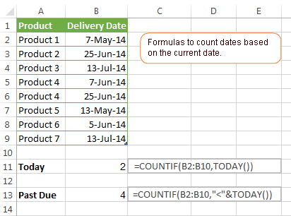
Apart from these common usages, you can utilize the COUNTIF function in conjunction with specific Excel Date and Time functions such as TODAY() to count cells based on the current date.
| Criteria | Formula Example |
|---|---|
| Count dates equal to the current date. | =COUNTIF(A2:A10,TODAY()) |
| Count dates prior to the current date, i.e. less than today. | =COUNTIF(A2:A10,"<"&TODAY()) |
| Count dates after the current date, i.e. greater than today. | =COUNTIF(A2:A10,">"&TODAY()) |
| Count dates that are due in a week. | =COUNTIF(A2:A10,"="&TODAY()+7) |
| Count dates in a specific date range. | =COUNTIF(B2:B10, ">=6/1/2014")-COUNTIF(B2:B10, ">6/7/2014") |
Here is an example of using such formulas on real data (at the moment of writing today was 25-Jun-2014):
Excel COUNTIF with multiple criteria
In fact, Excel COUNTIF function is not exactly designed to count cells with multiple criteria. In most cases, you'd use its plural counterpart, the COUNTIFS function to count cells that match two or more criteria (AND logic). However, some tasks can be solved by combining two or more COUNTIF functions in one formula.
Count values between two numbers
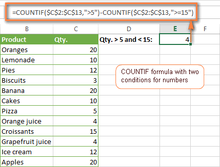
One of the most common applications of Excel COUNTIF function with 2 criteria is counting numbers within a specific range, i.e. less than X but greater than Y. For example, you can use the following formula to count cells in the range B2:B9 where a value is greater than 5 and less than 15.
=COUNTIF(B2:B9,">5")-COUNTIF(B2:B9,">=15")
How this formula works:
Here, we use two separate COUNTIF functions - the first one finds out how many values are greater than 5 and the other one gets a count of values greater than or equal to 15. Then, you subtract the latter from the former and get the desired result.
Count cells with multiple OR criteria
In situations when you want to get several different items in a range, add 2 or more COUNTIF functions together. Supposing, you have a shopping list and you want to find out how many soft drinks are included. To have it done, use a formula similar to this:
=COUNTIF(B2:B13,"Lemonade")+COUNTIF(B2:B13,"*juice")
Please pay attention that we've included the wildcard character (*) in the second criterion, it is used to count all kinds of juice on the list.
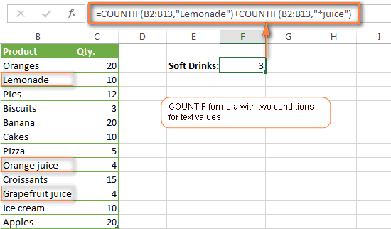
In the same manner, you can write a COUNTIF formula with several conditions. Here is an example of the COUNTIF formula with multiple OR conditions that counts lemonade, juice and ice cream:
=COUNTIF(B2:B13,"Lemonade") + COUNTIF(B2:B13,"*juice") + COUNTIF(B2:B13,"Ice cream")
For other ways to count cells with OR logic, please see this tutorial: Excel COUNTIF and COUNTIFS with OR conditions.
Using COUNTIF function to find duplicates and unique values
Another possible usage of the COUNTIF function in Excel is for finding duplicates in one column, between two columns, or in a row.
Example 1. Find and count duplicates in 1 column
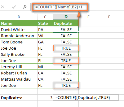
For example, this simple formula =COUNTIF(B2:B10,B2)>1 will spot all duplicate entries in the range B2:B10 while another function =COUNTIF(B2:B10,TRUE) will tell you how many dupes are there:
Example 2. Count duplicates between two columns
If you have two separate lists, say lists of names in columns B and C, and you want to know how many names appear in both columns, you can use Excel COUNTIF in combination with the SUMPRODUCT function to count duplicates:
=SUMPRODUCT((COUNTIF(B2:B1000,C2:C1000)>0)*(C2:C1000<>""))
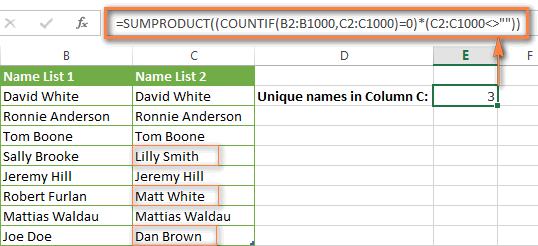
We can even take a step further and count how many unique names there are in Column C, i.e. names that do NOT appear in Column B:
=SUMPRODUCT((COUNTIF(B2:B1000,C2:C1000)=0)*(C2:C1000<>""))
Tip. If you want to highlight duplicate cells or entire rows containing duplicate entries, you can create conditional formatting rules based on the COUNTIF formulas, as demonstrated in this tutorial - Excel conditional formatting formulas to highlight duplicates.
Example 3. Count duplicates and unique values in a row
If you want to count duplicates or unique values in a certain row rather than a column, use one of the below formulas. These formulas might be helpful, say, to analyze the lottery draw history.
Count duplicates in a row:
=SUMPRODUCT((COUNTIF(A2:I2,A2:I2)>1)*(A2:I2<>""))
Count unique values in a row:
=SUMPRODUCT((COUNTIF(A2:I2,A2:I2)=1)*(A2:I2<>""))

Excel COUNTIF - frequently asked questions and issues
I hope these examples have helped you to get a feel for the Excel COUNTIF function. If you've tried any of the above formulas on your data and were not able to get them to work or are having a problem with the formula you created, please look through the following 5 most common issues. There is a good chance that you will find the answer or a helpful tip there.
1. COUNTIF on a non-contiguous range of cells
Question: How can I use COUNTIF in Excel on a non-contiguous range or a selection of cells?
Answer: Excel COUNTIF does not work on non-adjacent ranges, nor does its syntax allow specifying several individual cells as the first parameter. Instead, you can use a combination of several COUNTIF functions:
Wrong: =COUNTIF(A2,B3,C4,">0")
Right: =COUNTIF(A2,">0") + COUNTIF(B3,">0") + COUNTIF(C4,">0")
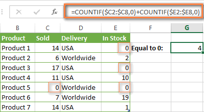
An alternative way is using the INDIRECT function to create an array of ranges. For example, both of the below formulas produce the same result you see in the screenshot:
=SUM(COUNTIF(INDIRECT({"B2:B8","D2:C8"}),"=0"))
=COUNTIF($B2:$B8,0) + COUNTIF($C2:$C8,0)
2. Ampersand and quotes in COUNTIF formulas
Question: When do I need to use an ampersand in a COUNTIF formula?
Answer: It is probably the trickiest part of the COUNTIF function, which I personally find very confusing. Though if you give it some thought, you'll see the reasoning behind it - an ampersand and quotes are needed to construct a text string for the argument. So, you can adhere to these rules:
If you use a number or a cell reference in the exact match criteria, you need neither ampersand nor quotes. For example:
=COUNTIF(A1:A10,10)
or
=COUNTIF(A1:A10,C1)
If your criteria includes text, wildcard character or logical operator with a number, enclose it in quotes. For example:
=COUNTIF(A2:A10,"lemons")
or
=COUNTIF(A2:A10,"*") or =COUNTIF(A2:A10,">5")
In case your criteria is an expression with a cell reference or another Excel function, you have to use the quotes ("") to start a text string and ampersand (&) to concatenate and finish the string off. For example:
=COUNTIF(A2:A10,">"&D2)
or
=COUNTIF(A2:A10,"<="&TODAY())
If you are in doubt whether an ampersand is needed or not, try out both ways. In most cases an ampersand works just fine, e.g. both of the below formulas work equally well.
=COUNTIF(C2:C8,"<=5")
and
=COUNTIF(C2:C8,"<="&5)
3. COUNTIF for formatted (color coded) cells
Question: How do I count cells by fill or font color rather than by values?
Answer: Regrettably, the syntax of the Excel COUNTIF function does not allow using formats as the condition. The only possible way to count or sum cells based on their color is using a macro, or more precisely an Excel User-Defined function. You can find the code working for cells colored manually as well as for conditionally formatted cells in this article - How to count and sum Excel cells by fill and font color.
4. #NAME? error in the COUNTIF formula
Issue: My COUNTIF formula throws a #NAME? error. How can I get it fixed?
Answer: Most likely, you have supplied an incorrect range to the formula. Please check out point 1 above.
5. Excel COUNTIF formula not working
Issue: My COUNTIF formula is not working! What have I done wrong?
Answer: If you have written a formula which is seemingly correct but it does not work or produces a wrong result, start by checking the most obvious things such as a range, conditions, cell references, use of ampersand and quotes.
Be very careful with using spaces in a COUNTIF formula. When creating one of the formulas for this article I was on the verge of pulling my hair out because the correct formula (I knew with certainty it was right!) wouldn't work. As it turned out, the problem was in a measly space somewhere in between, argh... For instance, look at this formula:
=COUNTIF(B2:B13," Lemonade").
At first sight, there is nothing wrong about it, except for an extra space after the opening quotation mark. Microsoft Excel will swallow the formula just fine without an error message, warning or any other indication, assuming you really want to count cells containing the word 'Lemonade' and a leading space.
If you use the COUNTIF function with multiple criteria, split the formula into several pieces and verify each function individually.
And this is all for today. In the next article, we will explore several ways to count cells in Excel with multiple conditions. Hope to see you next week and thanks for reading!
 by
by
1038 comments
Hi,
I have Year in Column A (from 2005-2012), names of countries in Column B (like India, Australia, England, South Africa, etc.) and whether they "Win" or "Loss" in Column C. How do I use the Countif function to determine how many times India Won in total?
Vani:
Not sure about using COUNTIF. You can use COUNTIFS like this:
=COUNTIFS(A20:A27,"India,C20:C27,"Win")
Thanks a lot. It full fill my requirement.
=COUNTIF(IF((B2:B1000="India")+(C2:C1000="Win")=2;1);1)
={COUNTIF(IF((B2:B1000="India")+(C2:C1000="Win")=2;1);1)}
Remember, it is an array formula. Control+Shift+Enter
How can I use COUNTIF to check for duplicated entries in excel?
For example, if I have this the file below, how can CountIF show where the same STAN duplicates.
STAN Output
1234
2345
1234
5678
890
5678
6930
Edozie:
Where the STAN data is in A2:A8 the formula is:
=COUNTIF($A$2:$A$8,A2)>1 then copy it down the column.
Hi All,
=COUNTIFS(G:G, "12345",F:F, "Entry",E:E, "=500")
This formula counts well for the occurrence of the number 12345 with respect to the matching value in column E and F as mentioned in the formula.
But to make the formula worked for the next number below 12345, how will I point the next cell in this formula for the column G.
Basically I need mention the cell (G) instead of number in this formula. Tried many ways.. cudnt win.
Please help.
How to compare a condition between two table using COUNTIF function?
I mean suppose I have a column containing 'responsible party' name and another one 'rectification status'. How can I search for a condition between them using COUNTIF function?
I would like to make count of repeats in a column where another cell is blank.
Example
Number of times orange repeating where price of orange is $0.5
Another example
Number of times persons visited Dubai from Japan
Name Visited to from which country
ABC1 Dubai Japan
ABC2 Paris Japan
ABC3 Dubai China
ABC4 London Japan
ABC5 Dubai Japan
Here the answer is 2
Hey would anyone know how to use COUNTIF to compare two columns of data - dates, only counting IF the first column date is proir to the second? 30,000 data points so I cannot do it manually
Nick:
I think this is what you're looking for:
=COUNTIF(E6,">"&D6)
Where the dates are in columns E and D beginning in row 6 enter this in column F.
IFEOLUWA AKINNLO W/D ENGINEER
RAWLINGS U UWUIM BRC OPERATOR
JIMOH ISHMAEL AD W/D OPERATOR
AKANDU OKECHUKWU ELE Electrician
HENRY EYO DAVIS ELE Electrician
JOHN ETIM W/D OPERATOR
FRANKLIN IGHOROD ELE HOD
LASISI OLADIPUPO ELE D.G OP
ALEX ADEWOLE W/D OPERATOR
JIMOH RASAQ W/D OPERATOR
ADELEKE KAZEEM BRC OPERATOR
I WANT TO COUNT HOW MANY OPERATOR PRESENT DATE WISE. USING COUNTIF FUNCTION.
Dillip:
If the data is in the range A2:C27 the formula in D2 looks like:
=COUNTIF(A2:C27,"Operator")
For some reason the COUNTIF formula with dates isn't working on my spreadsheet. Say I have a list of dates in M/DD/YYYY format across multiple rows and columns. I want to use a formula to count how many of those dates fall into a particular week.
A B C D
1 4/26/2018 5/08/2018 5/15/2018 5/17/2018
2 4/26/2018
3 4/24/2018
4 4/26/2018 5/15/2018
5 4/24/2018
6 4/30/2018 5/16/2018
7 4/23/2018 4/30/2018 5/17/2018 5/14/2018
=COUNTIFS(A1:D7,">=&4/20/2018",A1:D7,"<&4/30/2018")
It should return 7, right? So why is it returning 13? I use the "&" because otherwise the value returns a 0. I'd appreciate the help.
Jon:
Does your Excel version support COUNTIFS? I use COUNTIFS for this and got the correct number which is 6.
=COUNTIFS(O23:R29,">=4/20/18",O23:R29,"<4/30/18")
When I changed the second criteria to be "<=4/30/18" the result is 8.
I'm working on a project and need to use greather or lesser than in the same Countif statement, can anyone help me can't seem to get it right.
Hi,
I'm trying to count if there was growth in a period and how much time the growth has sustained. So I need to start my count in a values greater than 0 to determine the length of time. My problem is, starting a count on the first negative number in a column determined by time, not counting every positive number in the same time series.
So I was wondering if and how you can set the criteria of COUNTIF so that one row equals another? Meaning I want to count B2:B100 if it equals A2:A100, in other words counting how many times column B equals column A in the same row.
In column C, I would add an if statement.
if(A2=B2,1,0) then AutoSum (or countif) column C.
Just found a better (quicker) way!!!
=SUMPRODUCT(0+(A2:A15=B2:B15))
Thanks, Barry! https://superuser.com/a/846065
I'm having trouble with a formula. I have =IF(COUNTIF(C2:C6,C2)=5,"YES","NO") and it works beautifully, except that I also need the result cell to remain blank if any of the cells C2:C6 are left blank. Help?
Hello
"If you want to count cells that contain an actual operator as part of the cell's contents, i.e. the characters ">", "<" or "=", then use a wildcard character with the operator in the criteria." It saved my life. Thank you
I'm trying to be able to take a column and count unique values (non-duplicates) and not count blanks. Haven't found the formula yet.
Ex. We assign ID numbers to each rqst submitted. I keep track on a spreadsheet. Each # may be used for multiple locations so they can appear more than once. I want to know how many unique ID#s I have and not count the blank cells (that are holding for new data to be entered).
Hi Can you assist,
I am using a countif formula and want to include indirect to count the number of "P" between 2 dates. I have this formula working but cant seem to get to work using indirect as get #value I want to use indirect as I have several similar sheets and just want 1 summary page.
Working formula not using indirect
=COUNTIFS(Sample!6:6,">="&B5,Sample!6:6,"="&B5),(INDIRECT("'"&$G$2&"'!"&$C6,"<="&C5),(INDIRECT("'"&$G$2&"'!"&$C8),I$7)))
G2=Sheetname which one is called sample
C6=6:6
C8=8:8
B5=From date
B6=To date
I7=P
Thanks
Matt
how do I get countif to count the value in a cell, i.e. if the cell references another cell or is a formula, "=H40" countif will not count the value in the cell, but only what is written in the cell. How do I work around this???
will yes counties does work on some formulas but not the one I am interested in
=COUNTIFS($H$50:$L$50,"=10")
will not count the output of
=TEXTJOIN("",TRUE,IFERROR(MID(H49,ROW(INDIRECT("1:100")),1)+0,""))
there are values in the cells that countif just does not see and all I get is zero.
found the problem numbers were being stored as text
Hi,
Need to count the days in Excel between two values in the same column.
For EX: How to count the value between less than 15 and greater than 30 days
please help... my professor asked as to count the name of anne so we make the formula =countif(A1:A12,"*anne*") but we need to make the string color green when the excel counts the name anne... what formula should we use? please i need answer in this confusing activity
Hi Paula,
To color cells or entire rows based on a cell value, you need to create a conditional formatting rule with a formula. In your case, the formula is as follows:
=SEARCH("anne", $A1)>0
The detailed steps to create a rule can be found here:
How to create a conditional formatting based on formula
i want to fine a value for a cell based on database
number value need ?
5 1 5 what is value
8 2
2 3
Hello, Sameer,
It looks like the VLOOKUP function will work for you.
Please find more information about VLOOKUP in this article.
Helllo - Please can you assist.
I am currently using the following formula and when there is nothing to display it shows a 0 how do I change the formula to show blank instead of 0
=COUNTIF(Table1113[@[CCN1]:[Plant & Appliances in Non Domestic Premises]],">"&TODAY())
many thanks
I would use the following to hide 0 results:
=if(COUNTIF(Table1113[@[CCN1]:[Plant & Appliances in Non Domestic Premises]],">"&TODAY())=0,"",COUNTIF(Table1113[@[CCN1]:[Plant & Appliances in Non Domestic Premises]],">"&TODAY()))
I am sure there are better answers than this, but it works for me.
Please help with my formula. I'm trying to get a total number in a cell based on text in a cell range (2 different parameters). My formula is as follows: =IF(COUNTIF(G3:G30, "Complete") < 1,(G3:G30, "Terminated") < 1,0, COUNTIF(G3:G30, "Complete")(G3:G30, "Terminated")) It is not working correctly. Any idea what I'm doing wrong? Thank you.
HELP PLS! I have a list of dates in Coulmn L and then a list of dates in Cloumn M. I want to be able calculate network days between L:L and M:M and if the difference is 3 don’t count. I then want to sum all the 1’s! I would like to do this all in one formula and without a helper column if possible. I have over the 1000 dates in column L and the same in coulmn M. Is this possible?
how can i use wild cards for numbers
I have 2 columns of data. Column A contains a date. Column B contains a temperature. Temperature measurements are made several times each day, so several rows will have the same date. I'm trying to determine how many unique days a specific temperature is reached. So, if a temperature is reached several times during the same day, it should only count as "1" occurrence.
Hi Steve! I have the exact same problem! Did you ever figure out how to do it?
Hello!
Please check out the following article on our blog, it’ll be sure to help you with your task: Count unique values with criteria and How to find unique values in Excel 2019, 2016 and earlier and How to count unique values in a column
If you have other questions, don't hesitate to ask.
I'm trying to set formula to keep track of wire by feet. B2 does not have a figure but will have one and B2 will change as wire is depleted. I want B2 to subtract entries in cells B3:B27 and show the balance of feet on hand in B2. I've put in formulas for subtracting but I can't put a formula in B2 while keeping the balance of wire in that same cell B2. HELP!
i want count for example how many (+) in an excel function in a cell
A1=4+5+6+7
so the count will be 3
is there a a function for that ?
or to count how many characters will be calculated
for the same example it will be 4
PLEASE PLEASE HELP!
If I want to count or sum a COLUMN, I can do =sum(F:F) for column F
Let's say cell A1 has F in it,
How can I reference A1 to do sum (so I can change that cell to do different columns like G, H, I, J).
I tried like =sum(&A1&:&A1&) but that doesn't help - I was hoping that would calculate as = sum(F:F)
Thanks!!!!
Hello,
Please try the following formula:
=SUM(INDIRECT(A1&":"&A1))
Hope it will help you.
Hello,
could you please help to fix my formula? something is not working here
=COUNTIFS($K$20:$K$734,"????????",$D$20:$D$734,"*.08.*")
where i have a table for date in text format (.08.), and another column where added some text. basically i need count how many cases in column K from the 8th month
Hello,
Actually, your formula for is correct, if it doesn't work, most likely there's something wrong in your table.
If you still require our assistance, please send us your workbook with the data and the result you expect to get to support@ablebits.com. Please don't worry if you have confidential information there, we never disclose the data we get from our customers and delete it as soon as the problem is resolved.
Don't forget to include the link to this comment into your email.
We'll look into your task and try to help.
I would like to count non-empty cells, but using the count if formula, it also counts the empty ones because they have a formula that return a value of nothing/blank/empty. How to make excel not to count these formulated empty cells?
Hello,
Please try the following formula:
=SUMPRODUCT(--(A:A<>""))
Hope it will help you.
Need Help
Data
1 2 3 4
Alpha 1 Alpha 3 ? ? ?
Beta 1 Beta ? ? ? ?
Gama 1 Gama ? ? ? ?
Beta 2
Gama 3
Gama 4 Formullae required How "3" Comes In Alpha 1
Alpha 1
Beta 2
Gama 1
Beta 4
Gama 4
Beta 3
Beta 4
Gama 1
Gama 2
Alpha 1
Beta 1
Hello,
For me to understand the problem better, please send me a small sample workbook with your source data and the result you expect to get to support@ablebits.com. Please don't worry if you have confidential information there, we never disclose the data we get from our customers and delete it as soon as the problem is resolved.
Please also don't forget to include the link to this comment into your email.
I'll look into your task and try to help.
81150001% is not available at the moment ?
Hello, I want to count qualifications. Column A has the number of days a qualification is good for, Column B has the date the qualification was completed. I want to take today's date - date qualification completed and count if it is less than the day value in Column B. Can you help?
Hello,
For me to understand the problem better, please send me a small sample workbook with your source data and the result you expect to get to support@ablebits.com. Please don't worry if you have confidential information there, we never disclose the data we get from our customers and delete it as soon as the problem is resolved.
Please also don't forget to include the link to this comment into your email.
I'll look into your task and try to help.
I need a formula with 3 conditions
count if column AS = "sold", column B = "x" and column J = "y"
Hi!
You can count the number of values that match the three criteria with the COUNTIFS function. Read this article: How to use Excel COUNTIFS and COUNTIF with multiple criteria. I hope my advice will help you solve your task.
Hi,
I have made a few unsuccessful attempts at making a formula to count pairs of cells based on specific criteria. I need to make a formula that will count how many pairs of cells meet the criteria. For example, if A1=2 and A34=1, then it will count that as 1 pair. Upwards of 12 pairs of cells will need to be accounted for, and I cannot select a range of cells because cell pairs are far apart.
Thanks for your help
Hello,
For me to understand the problem better, please send me a small sample workbook with your source data and the result you expect to get to support@ablebits.com. Please don't worry if you have confidential information there, we never disclose the data we get from our customers and delete it as soon as the problem is resolved.
Please also don't forget to include the link to this comment into your email.
I'll look into your task and try to help.
Hi,
I have a problem to find the proper formula for a sheet that trying to create.
In column A, I want the user to type the code of a customer.
That i have sorted with a data validation where only one entry is allowed.
However, only one entry per day. So the next day, the code should again be used.
CODE Date TIME
100 18/11/2017 14:55:36
100 18/11/2017 14:55:36
As you can see here, the code 100 can be used twice but that is what i would like to avoid.
The code 100 can only be used 1 time per day.
The sheet is for marketing purpose where the transportation expenses of a visiting customer is paid back. But only one time per day of course.
Is there a way, if possible with a data validation where i can enter a code to have a validation based upon a one time per day entry ?
Or one time 100 per day entry but the following day 100 is again usable but also then only 1 time.
I have been struggling with this issue now for 2 days and i simply can not find it.
Thanks ever so much for the support.
Eric
Hello,
Please create a custom Data Validation rule for column A using this formula:
=COUNTIFS(A:A,A1,B:B,B1)<=1
Hope it will help you.
Olá!
Gostaria fazer a contagem de células preenchidas (AI:AW), porém apenas das linhas indicadas por um critério (coluna I). É possível?
Muito obrigada!
Hello, Maria Pessoa,
Please try to use one of the following formulas:
=SUMPRODUCT(((I:I)="critério")*NOT(ISBLANK(AI:AW)))
Or
=COUNTIFS(I:I,"critério",AI:AI,"<>"&"")+COUNTIFS(I:I,"critério",AJ:AJ,"<>"&"")+COUNTIFS(I:I,"critério",AK:AK,"<>"&"")+COUNTIFS(I:I,"critério",AL:AL,"<>"&"")+COUNTIFS(I:I,"critério",AM:AM,"<>"&"")+COUNTIFS(I:I,"critério",AN:AN,"<>"&"")+COUNTIFS(I:I,"critério",AO:AO,"<>"&"")+COUNTIFS(I:I,"critério",AP:AP,"<>"&"")+COUNTIFS(I:I,"critério",AQ:AQ,"<>"&"")+COUNTIFS(I:I,"critério",AR:AR,"<>"&"")+COUNTIFS(I:I,"critério",AS:AS,"<>"&"")+COUNTIFS(I:I,"critério",AT:AT,"<>"&"")+COUNTIFS(I:I,"critério",AU:AU,"<>"&"")+COUNTIFS(I:I,"critério",AV:AV,"<>"&"")+COUNTIFS(I:I,"critério",AW:AW,"<>"&"")
Hope it will help you.
Attempting to use Countif to determine month, however data range has date stamps
data example:
Row A1 "01/11/2017 08:25:44"
Row A2 "31/10/2017 12:42:16"
attempted countif:
=COUNTIF(A1:A2,"nov") produces no result???
please advise
Hello, Rich,
Please try the following formula:
=SUMPRODUCT((MONTH(A1:A2)=11)*1)
Hope it will help you.
How do I create a formula that can work as a criteria range?
Here is an example.
COUNTIFS("T"&MATCH(W23,W:W,0)&":"&T23,T23,U$18:U23,U23,V$18:V23,V23,W$18:W23,W23)
Using countif i want count time 25:00:00 to 35:00:00. can tell me the formula to solve this???
I am trying to count the numbers that not equal in one column. for example
1
2
3
3
3
5
5
I am using count if but it's not working.
Hello, Sam,
if I understand your task correctly, this formula may help:
=SUM($A$1:$A$7*($A$1:$A$7<>OFFSET($A$1:$A$7,1,0))+IF($A$7=OFFSET($A$7,1,0),$A$7,0))
If it won't, and you need to exclude any number that appears more than once, feel free to try our Duplicate Remover add-in first, and then SUM function to sum the results.
Otherwise, you will need VBA code or a macro, but I'm afraid we won't be able to help you with those.
I realize this post is old and I might not get a response now, but I figure it's worth a shot since the original article helped me a lot.
I had started with the formula
=SUMPRODUCT((COUNTIF(F12:V2015,'Actividad (2) de LiCS'!C15:C2020)>0)*('Actividad (2) de LiCS'!C15:C2020""))
to count the number of unique names in a list that also occur in a list on another worksheet. I also wanted to know the number of such names associated with a particular date range, so I edited to
=SUMPRODUCT((COUNTIFS(D12:D2015,">"&(DATE(D10,1,1)),D12:D2015,"0)*('Actividad (2) de LiCS'!C15:C2020""))
and it worked great. But then I realized I also wanted to count the total number of names - even repeats - that occurred in both lists. I used the formula
{=SUMPRODUCT((COUNTIF('Actividad (2) de LiCS'!C15:C2020,F12:F2020)>0)*(F12:F2020""))}
to do so, and also worked great. But when I try to make similar "countifs" edits to specify date ranges, it returns a #VALUE! error. The edited formula I'm getting the error on is
{=SUMPRODUCT((COUNTIFS(D12:D2020,">"&(DATE(D10,7,1)),D12:D2020,"0)*(F12:F2020""))}
Any advice?
Thanks in advance!
~Marissa
Hi, Please see the following chart.
A B C D E
HOUSE 4 4 - HOUSE 4 4 - HOUSE
HOUSE 4 4 - HOUSE 3 - BOX
TOY 1 1 - TOY 1 2 - SHOE
HOUSE 4 4 - HOUSE 1 - TOY
SHOE 2 2 - SHOE 2
SHOE 2 2 - SHOE
SOCK 1 1 - SOCK
HOUSE 4 4 - HOUSE
BOX 3 3 - BOX 3
BOX 3 3 - BOX
BOX 3 3 - BOX
Column A is the item, column B is the count for each reoccurrence in column A, column C is =CONCATENATE(B1," - ",A1), column D counts and removes duplicates =IF(COUNTIF($B$1:B1,B1)=1,B1,"") and column E sorts and shows how many of each. The problem I am having is it only seems to count an item with a count of "1", only once so if there is more than 1 item with one occurrence, it only counts the first one. Can you tell me what I'm doing wrong?
My formulas are as follows:
Column A (no formula)
Column B =COUNTIF($A$1:$A$11,A1)
Column C =CONCATENATE(B1," - ",A1)
Column D =IF(COUNTIF($B$1:B1,B1)=1,B1,"")
Column E =IF(ROW(A1)>COUNT($D$1:$D$11),"",INDEX($C$1:$C$11,MATCH(LARGE($D$1:$D$11,ROW(A1)),$D$1:$D$11,0)))
Thanks!
Scott
Svetlana,
I am trying to use COUNTIF to count the output of a formula, e.g. a cell that contains a formula. The formula is a nested =IF() function.
COUNTIF however doesn't seem to see the output. For example, if other cells meet certain criteria, the output is "D". When I then use COUNTIF to count the "D"s it returns 0.
I'm familiar with COUNTIFS but I am using COUNTIF in this way to measure time and create a Gantt chart that doesn't overlap processes. If one process is going on, the cell returns "D" (for delay) and I can count that delay, via COUNTIF.
So, can I count formula outputs via COUNTIF, or is there another way to count formula outputs and/or display them differently?
Thanks!!
Lucas
Hello, Lucas,
COUNTIF should work in your case perfectly, I'm afraid the problem lies in something else. Perhaps, it is the spaces around "D". We could suggest you better, if you sent us your file with the formula to support@ablebits.com. Don't forget to include the link to this comment in your email.
Please don't worry if you have confidential information in your document, we never disclose the data we get from our customers and delete it as soon as the problem is resolved.
I am trying to count certain text in a range of cells from another tab. I need to count "status" and "status date" as separate formulas for counts. I tried this but didn't work: =COUNTIF('690-JHC3 Ven 600-699'!F4:F10001,"*STATUS*")and the other =COUNTIF('690-JHC3 Ven 600-699'!F4:F10001,"*STATUS DATE*")
Appreciate the help - thanks
Hi Kim,
Try this
=COUNTIF('690-JHC3 Ven 600-699'!F4:F10001,"*"&"STATUS"&"*")
This should ensure that STATUS is counted no matter what is before or after the word.
HI THERE ,
I WANT TO CALCULATE NO OF UNIQUE ALPHANUMERIC CHARACTER(EXMP.I-INKOL17000522 OR IN17000523) MONTH WISE REMOVING DUPLICATE .NEED TO USE ONE DROP DOWN LIST OF MOTHS TO GET MONTH WISE TOTAL NO OF OCCURRENCE.
PLS HELP
Hi, Sammie,
I'm sorry, it's difficult to help you with a formula since we don't know how your data is stored.
However, If I understand your task correctly, first of all you need to sum unique values. You can do that by following the instructions from this article.
And then, using these results, you create a drop-down list.
Hope you'll find this information helpful!
Hello Svetlana,
I have been reading through your website and can't see the answer to what I thought would be a fairly common question. Can you please help?
I have a created a spreadsheet of people from 10 different work teams. The team names are in column E. Columns J through AG are a range of competencies people are required to complete.
For each person’s row, where they have completed the competencies matching the column heading I would like to record the date they completed that particular competency.
For example:
. A B C D
1 Name Team Competency 1 Competency 2
2 John Red 10/08/17 16/07/17
3 James Red 16/07/17
4 Bob Red 16/07/17
5 Sara Blue 16/07/17
6 Gale Blue 11/07/17
7 Alice Blue
8 Dave Blue 16/07/17
9 Jane Green 11/07/17
10 Blair Green
What I cannot work out is how to create a formula to count the number of people from the Blue team (or any specific team) who have completed Competency 1.
Ideally the results of these formulas will be used to create a table similar to this:
Team Com 1 completed Com 2 completed
Red 2 2
Blue 3
Green 1
Thank you for your assistance.
CS
Hi,
I want to know from you that how can I count the two cell data at a time like:
colA
OC TC
OC SC
OC SC
OC EC
OC TC
OC ST
R1 SC
R1 TC
R1 SC
R1 TC
I want to know for OC how many TC of SC and for R1 how many TC or SC Like ------------
TANK YOU.
BR,
Achira
Hi there , I have a simple table I did not set it up as pivot table. First row are dates and under each date there are columns with stock symbols( 10-50 symbols under each date average ). I am using a count if formula in conditional formatting to determine how many times each stock symbol appears in my table =COUNTIF($A$2:$Z$100,A2)=5 it is a relative reference and I ask a certain color for cells that meet criteria . I set up the range to be same as in formula A2:Z100 Every day I add up symbols and some times I delete columns that are dated more than 2 months ago. The problem is that every day after I add up a new column the range that formula apply to is changing so I have to manually set it up ( conditional formatting/manage rule /this worksheet/applies to )
How can I overcome this problem ? Basically I was looking to add up every day a column and symbols that meet criteria of countif formula to be highlighted let say green
Hello,
I am trying to write a formula to count the number of calls for the first meeting from two separate spreadsheets. I was able to count the total calls for all the meeting but I can figure out how many calls for the first meeting and 2nd meeting and so on.
My first Spreadsheet is the meeting sheet and I have customer column, created date. the second sheet is the phone call sheet with customer name and the date (each call create one date)
I used countif formula to count if the customer exist in the phone list then count the number of call but this formula only gave me the total then I added additional count if formula to say if the phone call date less than the meeting created date then count those number but all I got an error value. Can you help?
Thank you,
LE
Hello,
Please I want to group items but want to write a function so that all those who qualify are assigned 1 and those who do not qualify are assigned 0. Please help
Does Countif work with Frequency? I've found an example to count how many different values there are in a large array as the following
= SUM( --(FREQUENCY(A1:A1000,A1:A1000)>0))
so I thought that COUNTIF should work to
= COUNTIF(FREQUENCY(A1:A1000,A1:A1000),">0")
However, the formula is not accepted. Do you know if there is a limitation in the type of argument?