Microsoft Excel provides several functions purposed for counting different kinds of cells, such as blanks or non-blanks, with number, date or text values, containing specific words or character, etc.
In this article, we will focus on the Excel COUNTIF function that is purposed for counting cells with the condition you specify. First, we will briefly cover the syntax and general usage, and then I provide a number of examples and warn about possible quirks when using this function with multiple criteria and specific types of cells.
In essence, COUNTIF formulas are identical in all Excel versions, so you can use the examples from this tutorial in Excel 365, 2021, 2019, 2016, 2013, 2010 and 2007.
COUNTIF function in Excel - syntax and usage
Excel COUNTIF function is used for counting cells within a specified range that meet a certain criterion, or condition.
For example, you can write a COUNTIF formula to find out how many cells in your worksheet contain a number greater than or less than the number you specify. Another typical use of COUNTIF in Excel is for counting cells with a specific word or starting with a particular letter(s).
The syntax of the COUNTIF function is very simple:
As you see, there are only 2 arguments, both of which are required:
- range - defines one or several cells to count. You put the range in a formula like you usually do in Excel, e.g. A1:A20.
- criteria - defines the condition that tells the function which cells to count. It can be a number, text string, cell reference or expression. For instance, you can use the criteria like these: "10", A2, ">=10", "some text".
And here is the simplest example of Excel COUNTIF function. What you see in the image below is the list of the best tennis players for the last 14 years. The formula =COUNTIF(C2:C15,"Roger Federer") counts how many times Roger Federer's name is on the list:
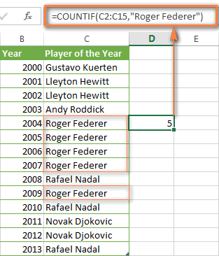
Note. A criterion is case insensitive, meaning that if you type "roger federer" as the criteria in the above formula, this will produce the same result.
Excel COUNTIF function examples
As you have just seen, the syntax of the COUNTIF function is very simple. However, it allows for many possible variations of the criteria, including wildcard characters, the values of other cells, and even other Excel functions. This diversity makes the COUNTIF function really powerful and fit for many tasks, as you will see in the examples that follow.
COUNTIF formula for text and numbers (exact match)
In fact, we discussed the COUNTIF function that counts text values matching a specified criterion exactly a moment ago. Let me remind you that formula for cells containing an exact string of text: =COUNTIF(C2:C15,"Roger Federer"). So, you enter:
- A range as the first parameter;
- A comma as the delimiter;
- A word or several words enclosed in quotes as the criteria.
Instead of typing text, you can use a reference to any cell containing that word or words and get absolutely the same results, e.g. =COUNTIF(C1:C9,C7).
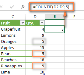
Similarly, COUNTIF formulas work for numbers. As shown in the screenshot below, the below formula perfectly counts cells with quantity 5 in Column D:
=COUNTIF(D2:D9, 5)
In this article, you will find a few more formulas to count cells that contain any text, specific characters or only filtered cells.
COUNTIF formulas with wildcard characters (partial match)
In case your Excel data include several variations of the keyword(s) you want to count, then you can use a wildcard character to count all the cells containing a certain word, phrase or letters as part of the cell's contents.
Suppose, you have a list of tasks assigned to different persons, and you want to know the number of tasks assigned to Danny Brown. Because Danny's name is written in several different ways, we enter "*Brown*" as the search criteria =COUNTIF(D2:D10, "*Brown*").
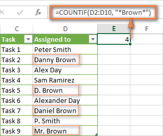
An asterisk (*) is used to find cells with any sequence of leading and trailing characters, as illustrated in the above example. If you need to match any single character, enter a question mark (?) instead, as demonstrated below.
Tip. It is also possible to use wildcards with cell references with the help of the concatenation operator (&). For example, instead of supplying "*Brown*" directly in the formula, you can type it in some cell, say F1, and use the following formula to count cells containing "Brown": =COUNTIF(D2:D10, "*"&F1&"*")
Count cells beginning or ending with certain characters
You can use either wildcard character, asterisk (*) or question mark (?), with the criterion depending on which exactly result you want to achieve.
If you want to know the number of cells that start or end with certain text no matter how many other characters a cell contains, use these formulas:
=COUNTIF(C2:C10,"Mr*") - count cells that begin with "Mr".
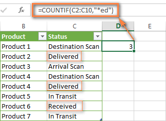
=COUNTIF(C2:C10,"*ed") - count cells that end with the letters "ed".
The image below demonstrates the second formula in action:
If you are looking for a count of cells that start or end with certain letters and contain the exact number of characters, you use the Excel COUNTIF function with the question mark character (?) in the criteria:
=COUNTIF(D2:D9,"??own") - counts the number of cells ending with the letters "own" and having exactly 5 characters in cells D2 through D9, including spaces.
=COUNTIF(D2:D9,"Mr??????") - counts the number of cells starting with the letters "Mr" and having exactly 8 characters in cells D2 through D9, including spaces.
Tip. To find the number of cells containing an actual question mark or asterisk, type a tilde (~) before the ? or * character in the formula. For example, =COUNTIF(D2:D9,"*~?*") will count all cells containing the question mark in the range D2:D9.
Excel COUNTIF for blank and non-blank cells
These formula examples demonstrate how you can use the COUNTIF function in Excel to count the number of empty or non-empty cells in a specified range.
COUNTIF not blank
In some Excel COUNTIF tutorials and other online resources, you may come across formulas for counting non-blank cells in Excel similar to this one:
=COUNTIF(A1:A10,"*")
But the fact is, the above formula counts only cells containing any text values including empty strings, meaning that cells with dates and numbers will be treated as blank cells and not included in the count!
If you need a universal COUNTIF formula for counting all non-blank cells in a specified range, here you go:
Or
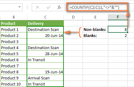
This formula works correctly with all value types - text, dates and numbers - as you can see in the screenshot below.
COUNTIF blank
If you want the opposite, i.e. count blank cells in a certain range, you should adhere to the same approach - use a formula with a wildcard character for text values and with the "" criteria to count all empty cells.
Formula to count cells not containing any text:
Since an asterisk (*) matches any sequence of text characters, the formula counts cells not equal to *, i.e. not containing any text in the specified range.
Universal COUNTIF formula for blanks (all value types):
The above formula correctly handles numbers, dates and text values. For example, here's how you can get the number of empty cells in the range C2:C11:
=COUNTIF(C2:C11,"")
Please be aware that Microsoft Excel has another function for counting blank cells, COUNTBLANK. For instance, the following formulas will produce exactly the same results as the COUNTIF formulas you see in the screenshot above:
Count blanks:
=COUNTBLANK(C2:C11)
Count non-blanks:
=ROWS(C2:C11)*COLUMNS(C2:C11)-COUNTBLANK(C2:C11)
Also, please keep in mind that both COUNTIF and COUNTBLANK count cells with empty strings that only look blank. If you do not want to treat such cells as blanks, use "=" for criteria. For example:
=COUNTIF(C2:C11,"=")
For more information about counting blanks and not blanks in Excel, please see:
COUNTIF greater than, less than or equal to
To count cells with values greater than, less than or equal to the number you specify, you simply add a corresponding operator to the criteria, as shown in the table below.
Please pay attention that in COUNTIF formulas, an operator with a number are always enclosed in quotes.
| Criteria | Formula Example | Description |
|---|---|---|
| Count if greater than | =COUNTIF(A2:A10,">5") | Count cells where value is greater than 5. |
| Count if less than | =COUNTIF(A2:A10,"<5") | Count cells with values less than 5. |
| Count if equal to | =COUNTIF(A2:A10,"=5") | Count cells where value is equal to 5. |
| Count if not equal to | =COUNTIF(A2:A10,"<>5") | Count cells where value is not equal to 5. |
| Count if greater than or equal to | =COUNTIF(C2:C8,">=5") | Count cells where value is greater than or equal to 5. |
| Count if less than or equal to | =COUNTIF(C2:C8,"<=5") | Count cells where value is less than or equal to 5. |
You can also use all of the above formulas to count cells based on another cell value, you will just need to replace the number in the criteria with a cell reference.
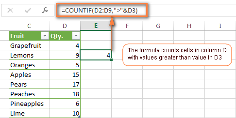
Note. In case of a cell reference, you have to enclose the operator in quotes and add an ampersand (&) before the cell reference. For example, to count cells in the range D2:D9 with values greater than a value in cell D3, you use this formula =COUNTIF(D2:D9,">"&D3):
If you want to count cells that contain an actual operator as part of the cell's contents, i.e. the characters ">", "<" or "=", then use a wildcard character with the operator in the criteria. Such criteria will be treated as a text string rather than a numeric expression. For example, the formula =COUNTIF(D2:D9,"*>5*") will count all cells in the range D2:D9 with contents like this "Delivery >5 days" or ">5 available".
Using Excel COUNTIF function with dates
If you want to count cells with dates that are greater than, less than or equal to the date you specify or date in another cell, you proceed in the already familiar way using formulas similar to the ones we discussed a moment ago. All of the above formulas work for dates as well as for numbers. Let me give you just a few examples:
| Criteria | Formula Example | Description |
|---|---|---|
| Count dates equal to the specified date. | =COUNTIF(B2:B10,"6/1/2014") | Counts the number of cells in the range B2:B10 with the date 1-Jun-2014. |
| Count dates greater than or equal to another date. | =COUNTIF(B2:B10,">=6/1/2014") | Count the number of cells in the range B2:B10 with a date greater than or equal to 6/1/2014. |
| Count dates greater than or equal to a date in another cell, minus x days. | =COUNTIF(B2:B10,">="&B2-"7") | Count the number of cells in the range B2:B10 with a date greater than or equal to the date in B2 minus 7 days. |
Apart from these common usages, you can utilize the COUNTIF function in conjunction with specific Excel Date and Time functions such as TODAY() to count cells based on the current date.
| Criteria | Formula Example |
|---|---|
| Count dates equal to the current date. | =COUNTIF(A2:A10,TODAY()) |
| Count dates prior to the current date, i.e. less than today. | =COUNTIF(A2:A10,"<"&TODAY()) |
| Count dates after the current date, i.e. greater than today. | =COUNTIF(A2:A10,">"&TODAY()) |
| Count dates that are due in a week. | =COUNTIF(A2:A10,"="&TODAY()+7) |
| Count dates in a specific date range. | =COUNTIF(B2:B10, ">=6/1/2014")-COUNTIF(B2:B10, ">6/7/2014") |
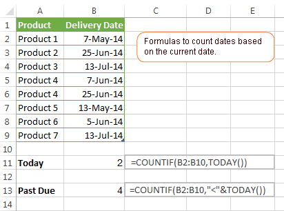
Here is an example of using such formulas on real data (at the moment of writing today was 25-Jun-2014):
Excel COUNTIF with multiple criteria
In fact, Excel COUNTIF function is not exactly designed to count cells with multiple criteria. In most cases, you'd use its plural counterpart, the COUNTIFS function to count cells that match two or more criteria (AND logic). However, some tasks can be solved by combining two or more COUNTIF functions in one formula.
Count values between two numbers
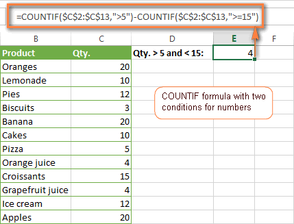
One of the most common applications of Excel COUNTIF function with 2 criteria is counting numbers within a specific range, i.e. less than X but greater than Y. For example, you can use the following formula to count cells in the range B2:B9 where a value is greater than 5 and less than 15.
=COUNTIF(B2:B9,">5")-COUNTIF(B2:B9,">=15")
How this formula works:
Here, we use two separate COUNTIF functions - the first one finds out how many values are greater than 5 and the other one gets a count of values greater than or equal to 15. Then, you subtract the latter from the former and get the desired result.
Count cells with multiple OR criteria
In situations when you want to get several different items in a range, add 2 or more COUNTIF functions together. Supposing, you have a shopping list and you want to find out how many soft drinks are included. To have it done, use a formula similar to this:
=COUNTIF(B2:B13,"Lemonade")+COUNTIF(B2:B13,"*juice")
Please pay attention that we've included the wildcard character (*) in the second criterion, it is used to count all kinds of juice on the list.
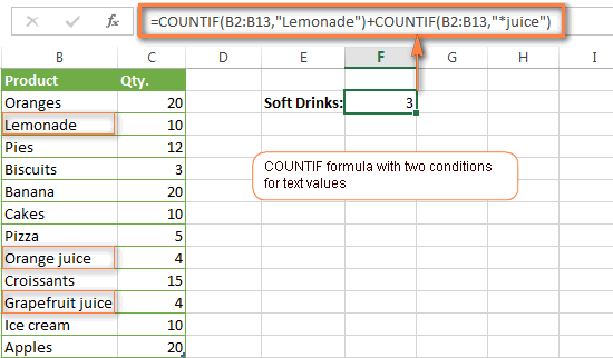
In the same manner, you can write a COUNTIF formula with several conditions. Here is an example of the COUNTIF formula with multiple OR conditions that counts lemonade, juice and ice cream:
=COUNTIF(B2:B13,"Lemonade") + COUNTIF(B2:B13,"*juice") + COUNTIF(B2:B13,"Ice cream")
For other ways to count cells with OR logic, please see this tutorial: Excel COUNTIF and COUNTIFS with OR conditions.
Using COUNTIF function to find duplicates and unique values
Another possible usage of the COUNTIF function in Excel is for finding duplicates in one column, between two columns, or in a row.
Example 1. Find and count duplicates in 1 column
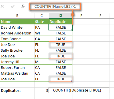
For example, this simple formula =COUNTIF(B2:B10,B2)>1 will spot all duplicate entries in the range B2:B10 while another function =COUNTIF(B2:B10,TRUE) will tell you how many dupes are there:
Example 2. Count duplicates between two columns
If you have two separate lists, say lists of names in columns B and C, and you want to know how many names appear in both columns, you can use Excel COUNTIF in combination with the SUMPRODUCT function to count duplicates:
=SUMPRODUCT((COUNTIF(B2:B1000,C2:C1000)>0)*(C2:C1000<>""))
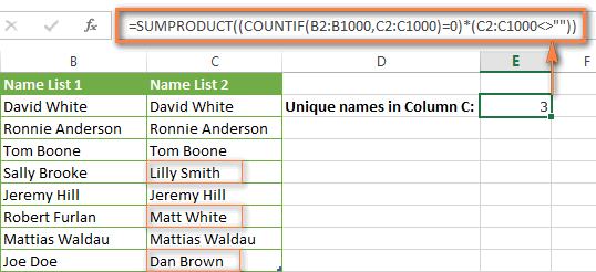
We can even take a step further and count how many unique names there are in Column C, i.e. names that do NOT appear in Column B:
=SUMPRODUCT((COUNTIF(B2:B1000,C2:C1000)=0)*(C2:C1000<>""))
Tip. If you want to highlight duplicate cells or entire rows containing duplicate entries, you can create conditional formatting rules based on the COUNTIF formulas, as demonstrated in this tutorial - Excel conditional formatting formulas to highlight duplicates.
Example 3. Count duplicates and unique values in a row
If you want to count duplicates or unique values in a certain row rather than a column, use one of the below formulas. These formulas might be helpful, say, to analyze the lottery draw history.
Count duplicates in a row:
=SUMPRODUCT((COUNTIF(A2:I2,A2:I2)>1)*(A2:I2<>""))
Count unique values in a row:
=SUMPRODUCT((COUNTIF(A2:I2,A2:I2)=1)*(A2:I2<>""))

Excel COUNTIF - frequently asked questions and issues
I hope these examples have helped you to get a feel for the Excel COUNTIF function. If you've tried any of the above formulas on your data and were not able to get them to work or are having a problem with the formula you created, please look through the following 5 most common issues. There is a good chance that you will find the answer or a helpful tip there.
1. COUNTIF on a non-contiguous range of cells
Question: How can I use COUNTIF in Excel on a non-contiguous range or a selection of cells?
Answer: Excel COUNTIF does not work on non-adjacent ranges, nor does its syntax allow specifying several individual cells as the first parameter. Instead, you can use a combination of several COUNTIF functions:
Wrong: =COUNTIF(A2,B3,C4,">0")
Right: =COUNTIF(A2,">0") + COUNTIF(B3,">0") + COUNTIF(C4,">0")
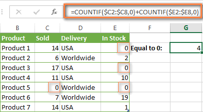
An alternative way is using the INDIRECT function to create an array of ranges. For example, both of the below formulas produce the same result you see in the screenshot:
=SUM(COUNTIF(INDIRECT({"B2:B8","D2:C8"}),"=0"))
=COUNTIF($B2:$B8,0) + COUNTIF($C2:$C8,0)
2. Ampersand and quotes in COUNTIF formulas
Question: When do I need to use an ampersand in a COUNTIF formula?
Answer: It is probably the trickiest part of the COUNTIF function, which I personally find very confusing. Though if you give it some thought, you'll see the reasoning behind it - an ampersand and quotes are needed to construct a text string for the argument. So, you can adhere to these rules:
If you use a number or a cell reference in the exact match criteria, you need neither ampersand nor quotes. For example:
=COUNTIF(A1:A10,10)
or
=COUNTIF(A1:A10,C1)
If your criteria includes text, wildcard character or logical operator with a number, enclose it in quotes. For example:
=COUNTIF(A2:A10,"lemons")
or
=COUNTIF(A2:A10,"*") or =COUNTIF(A2:A10,">5")
In case your criteria is an expression with a cell reference or another Excel function, you have to use the quotes ("") to start a text string and ampersand (&) to concatenate and finish the string off. For example:
=COUNTIF(A2:A10,">"&D2)
or
=COUNTIF(A2:A10,"<="&TODAY())
If you are in doubt whether an ampersand is needed or not, try out both ways. In most cases an ampersand works just fine, e.g. both of the below formulas work equally well.
=COUNTIF(C2:C8,"<=5")
and
=COUNTIF(C2:C8,"<="&5)
3. COUNTIF for formatted (color coded) cells
Question: How do I count cells by fill or font color rather than by values?
Answer: Regrettably, the syntax of the Excel COUNTIF function does not allow using formats as the condition. The only possible way to count or sum cells based on their color is using a macro, or more precisely an Excel User-Defined function. You can find the code working for cells colored manually as well as for conditionally formatted cells in this article - How to count and sum Excel cells by fill and font color.
4. #NAME? error in the COUNTIF formula
Issue: My COUNTIF formula throws a #NAME? error. How can I get it fixed?
Answer: Most likely, you have supplied an incorrect range to the formula. Please check out point 1 above.
5. Excel COUNTIF formula not working
Issue: My COUNTIF formula is not working! What have I done wrong?
Answer: If you have written a formula which is seemingly correct but it does not work or produces a wrong result, start by checking the most obvious things such as a range, conditions, cell references, use of ampersand and quotes.
Be very careful with using spaces in a COUNTIF formula. When creating one of the formulas for this article I was on the verge of pulling my hair out because the correct formula (I knew with certainty it was right!) wouldn't work. As it turned out, the problem was in a measly space somewhere in between, argh... For instance, look at this formula:
=COUNTIF(B2:B13," Lemonade").
At first sight, there is nothing wrong about it, except for an extra space after the opening quotation mark. Microsoft Excel will swallow the formula just fine without an error message, warning or any other indication, assuming you really want to count cells containing the word 'Lemonade' and a leading space.
If you use the COUNTIF function with multiple criteria, split the formula into several pieces and verify each function individually.
And this is all for today. In the next article, we will explore several ways to count cells in Excel with multiple conditions. Hope to see you next week and thanks for reading!
 by
by
1034 comments
halo i using COUNTIFS function but when i use it it appear #VALUE!
i just only write this
Location(title) JAN FEB
PgP1 ( WRITE HERE )
Hcp
Hello Mr Svetlana, i'm a doctor and i'm trying to figure out how to organize my colleagues data shift. I tried to use the "countif" formulas and it worked fine for normal shift that has to count 1 (stands for 1 turn of 6,3 hours) but i would like that excel will count a night shift as 2 (because the colleague that appear in the night line one time does 2 turns because he/she remains for 12 hours. How can i do that?
Thank you very much
Hi Paolo,
It's difficult for me to suggest an exact formula because I don't know how you identify night sifts. But you can use the following approach:
=COUNTIF(A:A, "night shift")*2
Hi!
I have a list of approximately 12000 rows with data. Column A has unique IDs, while column B has a date. How can I remove duplicate rows based on identical ID, only when there exist another date within 60 days of the first post?
123456 12.09.2015
123457 13.09.2015
123456 15.10.2015
123458 25.11.2015
123456 12.12.2015
In the example above, I want to get rid of the third line as it is within the 60 days from line 1. However, I want to retain line 5, since that is more than 60 days after line 1. Is it at all possible?
Sincerely,
Christoffer
Hello Christoffer,
I recommend you to add a combined column in the following way:
ID Date Combined
123456 9/12/2015 123456 more 60
123457 9/13/2015 123457 more 60
123456 10/15/2015 123456 more 60
123458 11/25/2015 123458 more 60
123456 12/12/2015 123456 less 60
Please see a workbook with an example here:
https://support.ablebits.com/blog_samples/excel-countif-examples_198.xlsx
Then you can use our Excel add-in that allows you to remove duplicate rows.
https://www.ablebits.com/excel-suite/find-remove-duplicates.php
Hi Svetlana,
Would it be possible to count a number of cells that contain numbers with letters? such as a list of number plates?
AV63 OEB
AV63 OEM
AV63 OEN
AV63 OER
AV63 OES
AV64 PYH
AV64 PYW
BJ13 LZW
BJ13 MGE
BV13 CZH
BV63 CGF
CK13 DKJ
FD13 KYJ
Thanks!
Hello Matt,
You can use the following function to extract only numbers from text string:
=SUMPRODUCT(MID(0&E5,LARGE(INDEX(ISNUMBER(--MID(E5,ROW($1:$25),1))* ROW($1:$25),0),ROW($1:$25))+1,1)*10^ROW($1:$25)/10)
Please see a workbook with an example here:
https://support.ablebits.com/blog_samples/excel-countif-examples_197.xlsx
I am counting rows that have unique values and also match multiple criteria, but the formula I have is coming up a view short each time. Using a helper worksheet on the same tab does not help:
I4 refers to a Warehouse ID = say "2A", and I need to count the unique bin locations referred to in E2:E7111. So for a specific warehouse, i need the number of unique bin locations in the array for warehouse 2A.
{=SUM(IF($A$1:$A$7111=I4,1/COUNTIF($E$2:$E$7111,$E$2:$E$7111)))}
Appreciate your eyes on this to see if I'd doing something wrong.
Thanks
David
Hello David,
If possible, please send a sample spreadsheet with the way your data and the expected results look to support@ablebits.com. Please include the name of the blog post and your comment. We'll do our best to assist you.
Hi Svetlana
Can I have a tab number in my countif formula e.g. =COUNTIF(C3:C46,"*C48*").
I am essentially trying to have a tab (in this case c48) that I can change the request in.
So for example if I change the content in c48 to OSS - it will count how many time OSS appears in my cell range of c3:c46.
Then if I change c48 to World - it will count how many times world appears in my cell range.
Thank you in advance
Hello
Can somebody help me in doing this in excel. I have a bunch of rows with 8 numbers in each row. I want to compare the numbers in the first row with the numbers of the second row. Then it gives me a count of how many numbers are the same. Then we move on to compare the numbers of the first row with the numbers of the third row and again it gives me a count of how many numbers are the same AND adds it to the result of the first comparison. …. And so on till we end up to the last row(i.ei 10th row).
For example:
Row 1 2 5 7 9 10
Row 2 6 4 2 11 5
Row 3 6 9 12 2 7
Row 4 8 1 4 11 6
Comparing the numbers in row1 to the numbers in row 2 results in 2 as the numbers 2 and 5 are in both rows. Then we compare the numbers in row1 with the numbers in row3 which will results with 3 as the numbers 2,7,9 are in both rows. Hence the new returned value will be 2(result from first row checking)+3(result from second row checking)=5
Then we compare the numbers in row1 with the numbers in row4 which will results with 0 as there are no matching numbers between the row1 and row4. Hence the new returned value will still be 5(result from first row checking)+3(result from second row checking)+ 0(result from forth row checking)=5
Now we start comparing the numbers of row2 with the numbers of the other rows and so on
thanks
I'm trying to count how many "Yes" in I2:I322, only if D2:322 equals "SSA"
=COUNTIFS(USA!D2:D322, "SSA",USA!I2:I322, "Yes")
It's only counting a subset of all the "Yes"s that qualify.
I figured out this formula is working. The problem is that it seemed it was wrong because of filtered rows. So, please ignore this question. Thanks :)
svethlen mam..
am going for analysing data in spreadsheet which is taken from rating questionair data. here is data like.
a
b
c
d
c
b
d
d
c
a
in want konw how many A.B.C.& D ' s in this coloum.. plz sugest me a formula for this problem...
Hi, I use =SUM(1/COUNTIF(M3:M100;M3:M100)) formula for calculate name in row and it is working without blank cell. but in this range I have some blank cell and formula is not working. Please help
Svetlana,
Is there any way to use an iteration of the countif fuction to match words on two different columns and give a total, but exclude if that specific word is on both columns.
Example Below. There are 4 columns A,B,C,D and if i use the countif and look for june on column A, it will give me a total of 1 which is found on A3.
What I want is a countif formula to look at column A and column C, and look for the word June and give me a total, but exclude from the total if the word june is in both columns, which would be 2 since C1 and C5 only show up once on both columns and A3 and C3 is exclude since they appear on both.
A B C D
1. march 2 June M
2. april T March 1
3. june 3 June G
4. july y july 6
5. May 5 June 4
=IF(G8-F8,"Partial","Full") - I want to add another text. Can help?
Let me ask u one .
what is the formula to count the redundancy of the value in a single cell with the range time?
e.g how many times , i write "N" In cell A1 From 2:30 to 2:45
Hi Svetlana,
I have a range of cells from F8:F65,to DB8:65 all with Values like "Pass" and "Fail". I want to capture the results of Pass in a formula using COUNTIF. My example is =SUM(COUNTIF(F8:F65,"Pass"),(COUNTIF(G8:G65,"Pass"),(COUNTIF(H8:H65,"Pass"))). But this is not working. It is working till the G8:G65, but later it is not working.
I know there are 5858 "Pass" in this range but want to capture this information in a cell without having to hardcode this.
Thanks and Regards,
KM
Hi, I want to filter the value for two column. The column has 3200 rows, same goes to the second column. So, now I want to filter the number of row for column A that have greater value than column B. Please, i really need your help. :'(
Hi
I have looked at the responses above but I can't see anything close to what I need. I have 3 columns. the first has office names and the second has PO numbers, the third has dates. The second column has unique and duplicate PO's. I would like to count the amount of uniquem then duplicate PO's from a certain office in a certain date range. i.e Cardiff between 1-2-15 and today.
Thanks
Hello Pete,
I added two auxiliary column.
Please see a workbook with an example here:
https://support.ablebits.com/blog_samples/excel-countif-examples_185.xlsx
Hi Svetlana,
Quick question on how to use the countif/countblank.
I have an excel spreadsheet where I need to determine the number of items in a column that are blank so I am using =countblank (A1:A94) but I have to continually change the range because if I do =countblank (A:A) I will get too many results.
So my question is which formula could I use to count blanks in all of A if column B = Yes
I figured it out after browsing the site some more.
For those wondering; here is the formula
=COUNTIFS(A:A,"",B:B,"YES")
i have a table with "count" formula on one column then an "expired" word on the other, i was thinking if there's a way which i could see that the number of "expired" units will be equal to the number as have been counted. wish i could have shown you my table. tnx
please help me i need to pass or fail a learner in a row from C6:O6, by getting 3x30s and 3x40s
THANX YAR
Hello, i'm trying to count the results to a survey i conducted and i need to graph very specific things.
What i want to do, in English, would be like:
If (column C)= Female, count how many times the word "weapons" is in column G
I don't know if it's there in the examples and i can't see it because i'm not used to Excel, or if it just can't be done.
Thanks for the tutorial though! I'm going to use some other things.
Hello Catalina,
Use the following formula:
=COUNTIFS(C1:C12,"Female",D1:D12,"weapons")
Please see a sample file:
https://support.ablebits.com/blog_samples/excel-countif-examples_180.xlsx
What do i need to do to count data that has a date less than today, but only count as far back a 2 weeks?
=countif(A23:a,""today -14??
Hi Matthew,
To count with 2 or more conditions, you need to use the COUNTIFS function:
=COUNTIFS(A1:A20, "<"&TODAY(), A1:A20,">="&TODAY()-14)
Dear Lidiya,
Can i calculate 00:01 to 00:59 mnts Greater than equal to 1 and 01:00 to 9:59 Greater than equa 2 how can i do it
thank
k sahoo
plz give me a example i can not under stood
Dear Mam/sir
Can i calculate 00:01 to 00:59 mnts equal -1 and01:00 to 9:59 euql 2 how can i do it
thank
k sahoo
Hi there - I am close to my solution but am stuck with my function. I have values of 1-7 that each number represents a certain type of "fail" for my employees in their audit. Each row in my sheet represents an employee and in their corresponding cell, there might be multiple reasons for them to fail an audit and sometimes the failed reason could occur twice in their audit. So, if Ben failed an audit only because of "insufficient financial information", then he would get a "1" in his corresponding cell, (where 1 corresponds to that particular fail). However if Donna failed due to "insufficient financial information" (1) and "MD referral guidelines not followed", (which corresponds to number 6)then on another case failed due to "1" again then she would have a "1,6,1" in her corresponding cell. So I have employee names in column A, then the fail results in column B. Then I have D1 labled "Fail Type" and E1 though K1 labeled 1 through 7. Then D2 labeled "count of Type" and starting with E2 through K2 I have the formula =COUNTIF($B$2:$B$5,"*"&E$1&"*")+COUNTIF($B$2:$B$5,E$1) in each cell - it will only count Donna's two "1's" in her cell, once. I need to have it count those both times they occur in Donna's so that in E2, it shows "3" instead of "2" as it does currently.
I'm sorry, it's a bit hard for me to understand your task. Please send a sample spreadsheet with the way your data and the expected results look to support@ablebits.com. Please include the name of the blog post and your comment. We'll do our best to assist you.
Hi, I am working from a formula on Excel's Student calendar template. The current formula is =IF(LEN(B14)=0,"",IF(COUNTIF(Assignments[Month],DATE(WkYear,WkMonthNum,B14))>0,"Assignment due!",""))
I would like to change the "true" value from "assignment due!" to whatever the contents are in the cell is that it found in the look up (i.e the name of the assignment).
I Can't figure out how to make that happen- can you assist?
Thanks for your help!
Hello Katie,
Can you please send the source data and the expected result to support@ablebits.com, so I will try to help.
Hello,
I just used your countif suggestions and think I'm doing something wrong because I'm not getting the correct value.
Here is the formula I used:
=COUNTIF(NexTrak!B2:B130, "Bariatric") + COUNTIF(NexTrak!C2:C130, "Washington")
However, instead of telling me the amount of clients in the Bariatric specialty in the state of Washington, it is adding them (most likely bc of the +). How would I use the Countif formula as a type of conditional formula. I actually only have 1 Bariatric Client in Washington and 39 Clients total in Washington.
hi svetlana,
pls i need help about COUNTIF or COUNtBLANKFunctions
How to count more blank cells separately from date for example 22.09.2015 we have 4 blank application . i trayed this but not work- =COUNTBLANK(S16:S39)-COUNTIF(S16:S39,B43 or =COUNTIF(S16:S39,""&"*")
22.09.2015
22.09.2015
22.09.2015
22.09.2015
22.09.2015
23.09.2015
23.09.2015
28.09.2015
28.09.2015
Hi Svetlana hope you can help me.
JOHN 6
JOHN -5
BARRY 10
BARRY 9
BARRY -7
ZACK 3
ZACK 4
ZACK -8
ZACK -10
JIM 1
JIM 2
Can i make a formula where the result is john 1 , berry 12 , zack -11 , jim 3.
so it needs to look at the first and see how many johns there are and then calculate all the numbers john has.
regards,
john
Hi Svetlana, how would i do countif for a scenario like this?
10
20
80
100 210
10
20
200 30
the countif formula should check the anything <=100 and add it.
like answers should be 210 and 30..the values of first 4 cells are added and next 2 cells are added...Thank you...
Hello Can You please help me
A B
1,1500 1600
2,1300 1300
3,400 300
AB i want B3 in Red color
this must done in repeated columns
Hello,
I want to COUNTIF a range A:B that is less than zero and out of that I want to pick how many are from Paris?
I can do the first part and count how many are less than zero but how do I pick from that how many are equal to Paris?
I seem to be able to do 2 elements in a statement but cannot add a third?
Carol.
Hi Carol,
To count cells with more than one criteria, you have to use the COUNTIFS function, as demonstrated in the following tutorial:
https://www.ablebits.com/office-addins-blog/excel-countifs-multiple-criteria/
I have 10 columns (1 row) of data like below:
A|B|C|D|E|F|G|H|I|J
1|0|7|5|0|1|2|3|5|4
I need to form a new colum with triplets of numbers from each row,
like this:
A |
107|
075|
750|
501|
012|
235|
354|
Number 107 is formed of each separate value from cels A,B,C
Number 075 is formed of each separate value from cels B,C,D
Number 750 is formed of each separate value from cels C,D,E
.
.
.
etc.
Can enyone help me to do it?
Hi George,
Please use a combination of CONCATENATE and INDEX functions:
=CONCATENATE(INDEX($1:$1,1,ROW()-1),INDEX($1:$1,1,ROW()-1+1),INDEX($1:$1,1,ROW()-1+2))
You can download a sample with this formula:
https://support.ablebits.com/blog_samples/excel-countif-examples_164.xlsx
Hi there -
I am looking for help.
I need a formula that will count the number of times "Strongly Agree" appears in column F only if there is a number greater than 0 in column AF
I tried using multiple countIF functions as well as trying a Vlookup and am hainv no luck.
Hello Liz,
Please use a COUNTIFS function (ending with 'S')
=COUNTIFS(F1:F10,A1,AF1:AF10,">0")
Applies criteria to cells across multiple ranges and counts the number of times all criteria are met.
https://support.office.com/en-us/article/COUNTIFS-function-dda3dc6e-f74e-4aee-88bc-aa8c2a866842
Hey Svetlana!
Well done! I can see you have been providing answers to people for over a year.
Have a wonderful day :)
I have 10 columns (1 row) of data like below:
A|B|C|D|E|F|G|H|I|J
1|0|7|5|0|1|2|3|5|4
I need to form a new row with triplets of numbers from each column,
like this:
A |
107|
075|
750|
501|
012|
235|
354|
Number 107 is formed of each separate value from cels A,B,C
Number 075 is formed of each separate value from cels B,C,D
Number 750 is formed of each separate value from cels C,D,E
.
.
.
etc.
Can enyone help me to do it?
Hello George,
You can use a combination of CONCATENATE and INDEX functions in the following way:
=CONCATENATE(INDEX($1:$1,1,ROW()-1),INDEX($1:$1,1,ROW()-1+1),INDEX($1:$1,1,ROW()-1+2))
Please see a workbook with an example here:
https://support.ablebits.com/blog_samples/excel-countif-examples_164.xlsx
Hi there,
Pls help me with this:
Trying to form separate column from array like this:
A B C D F G H I J (Excell rows)
1 2 3 2 0 2 4 3 7 (value)
A B C D E
123 (New value)
232 (New value)
320 .
202 .
024 .
243 .
437 .
Thanks in advance.
Hello George,
I'm sorry, it's a bit hard for me to understand your task. Could you please explain it in more detail? If possible, please send a sample spreadsheet with the way your data and the expected results look to support@ablebits.com. Please include the name of the blog post and your comment. We'll do our best to assist you.
Hi Svetlana,
Pls help me
I want to count "o" in J2:PB2 when E2 is greater than 8 (E2>8) .
Thank u :)
hey there, i wanted to sum or count a list, excluding some specific names. Like there is a fruit list and wanted to count/sum excluding apples and mangoes.
i have five brands in the sales list A/B/C/D/E, want to sum only A/D/E
hey there, i wanted to sum or count a list, excluding some specific names. Like there is a fruit list and wanted to count/sum excluding apples and mangoes.
Hello please am trying to play around to see if i can use COUNIF or COUNTIFS to make my formula to count P and PS as one and the same thing in my totals. Thank you so much for the rapid response
Hi Silvester,
You can add up 2 COUNTIF functions, like this:
=COUNTIF(range, "P") + COUNTIF(range, "PS")
=COUNTIF(I:I,""&"")
Column I contains formulas that return "", or a message, the message may vary. I am trying to count the messages, but the count returned is of cells containing a formula.
e.g. the formula ="" put in a cell will increment the count
This is in Excel 2013
Nice article, thanks!
I have two columns of data like below. I need to count the number of times the value in column A is greater than the one in column B. Is this possible using COUNTIF?
A | B
2 | 1
1 | 2
3 | 0
2 | 1
Result A > B: 3 times
Result B > A: 1 time
Hi Martin,
You would need an array formula to compare 2 ranges, like in the following example (except that you don't want the second condition):
https://www.ablebits.com/office-addins-blog/excel-array-formula-examples/#count-cells-condition
The formula could be similar to this, please remember it requires pressing Ctrl+Shift+Enter:
=SUM((A1:A10>B1:B10) * 1)
Thanks, that works great! This is the formula I’m using (in Google Sheets):
=ArrayFormula(SUM((Data!B2:B1000 > Data!C2:C1000) * 1))
Hi need to calculate how many times for particular month my in time is 9:30, 9:40, 8:20,10:20,9:50,..........in month end 9:50. Please suggest formula for how
Many days I have come late my office time is 9:00.
Hi Svetlana,
I have a table that looks something like this: (0 is blank)
A1 B1
high run
0 run
0 run
high run
0 run
0 run
0 run
0 run
0 run
high run
I want to count the number of "run"s that occurs in the cell +1 column and -1 row of the cell with the value "high". So in this example, the return value would be 2.
I am only able to count for one instance rather than the whole column. Can you please give any insights on writing the formula for this problem?
Thank you
Hi Svetlana,
I have a table that looks something like this:
high run
run
run
high run
run
run
run
run
run
high run
I want to count the number of "run"s that occurs in the cell +1 column and -1 row of the cell with the value "high". So in this example, the return value would be 2.
I am only able to count for one instance rather than the whole column. Can you please give any insights on writing the formula for this problem?
Thank you
I've got a table of data that I have then created a number of concatenated columns from. From example, in my data, I have lists of contract numbers, and the month in which those contracts were processed (in some cases, this is across more than one month). I have therefore added a concatenated column that combines the contract number and the month number (1 for January, etc).
I want to be able to find out the number of times each contract has occurred within each month so I have tried a simple countif formula that says =COUNTIF(A:A,C1). Column A contains the concatenated column and C1 is where I have the contract number and month number also concatenated for the countif to be based on. However, I get a zero every time even though I know that combination of contract and month number appear three times.
Is my problem because all parts of the formula are referring to concatanated fields?
Thanks for any help provided - it should be so simple but there must be some sort of limitation in Excel that is holding me back.
I should add that the maximum length of the concatenated contract/month field is 10 digits.
Hello;
I'm looking to set up a formula that will count all values in column A, when column B has a date of 2012?
Thank you!
Hi Grace,
If you want to sum the values in column A, then you can use a formula similar to this:
=SUMIFS(A1:A6, B1:B6, ">=1/1/2012", B1:B6,"<=12/31/2012")
Hey, i need your help for
Col 1 has Unique id ( Emp Code) and col 5 has date.
i need to find out whether a Emp Code has Visited for more then once in a days.
exp emp code 101 and Emp has Visited for more then twice a days in 2 place.
need to make report regarding Emp Visited on tht day