Microsoft Excel provides several functions purposed for counting different kinds of cells, such as blanks or non-blanks, with number, date or text values, containing specific words or character, etc.
In this article, we will focus on the Excel COUNTIF function that is purposed for counting cells with the condition you specify. First, we will briefly cover the syntax and general usage, and then I provide a number of examples and warn about possible quirks when using this function with multiple criteria and specific types of cells.
In essence, COUNTIF formulas are identical in all Excel versions, so you can use the examples from this tutorial in Excel 365, 2021, 2019, 2016, 2013, 2010 and 2007.
COUNTIF function in Excel - syntax and usage
Excel COUNTIF function is used for counting cells within a specified range that meet a certain criterion, or condition.
For example, you can write a COUNTIF formula to find out how many cells in your worksheet contain a number greater than or less than the number you specify. Another typical use of COUNTIF in Excel is for counting cells with a specific word or starting with a particular letter(s).
The syntax of the COUNTIF function is very simple:
As you see, there are only 2 arguments, both of which are required:
- range - defines one or several cells to count. You put the range in a formula like you usually do in Excel, e.g. A1:A20.
- criteria - defines the condition that tells the function which cells to count. It can be a number, text string, cell reference or expression. For instance, you can use the criteria like these: "10", A2, ">=10", "some text".
And here is the simplest example of Excel COUNTIF function. What you see in the image below is the list of the best tennis players for the last 14 years. The formula =COUNTIF(C2:C15,"Roger Federer") counts how many times Roger Federer's name is on the list:
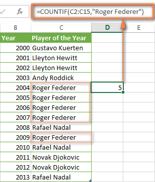
Note. A criterion is case insensitive, meaning that if you type "roger federer" as the criteria in the above formula, this will produce the same result.
Excel COUNTIF function examples
As you have just seen, the syntax of the COUNTIF function is very simple. However, it allows for many possible variations of the criteria, including wildcard characters, the values of other cells, and even other Excel functions. This diversity makes the COUNTIF function really powerful and fit for many tasks, as you will see in the examples that follow.
COUNTIF formula for text and numbers (exact match)
In fact, we discussed the COUNTIF function that counts text values matching a specified criterion exactly a moment ago. Let me remind you that formula for cells containing an exact string of text: =COUNTIF(C2:C15,"Roger Federer"). So, you enter:
- A range as the first parameter;
- A comma as the delimiter;
- A word or several words enclosed in quotes as the criteria.
Instead of typing text, you can use a reference to any cell containing that word or words and get absolutely the same results, e.g. =COUNTIF(C1:C9,C7).
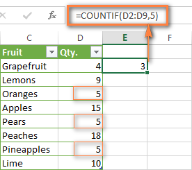
Similarly, COUNTIF formulas work for numbers. As shown in the screenshot below, the below formula perfectly counts cells with quantity 5 in Column D:
=COUNTIF(D2:D9, 5)
In this article, you will find a few more formulas to count cells that contain any text, specific characters or only filtered cells.
COUNTIF formulas with wildcard characters (partial match)
In case your Excel data include several variations of the keyword(s) you want to count, then you can use a wildcard character to count all the cells containing a certain word, phrase or letters as part of the cell's contents.
Suppose, you have a list of tasks assigned to different persons, and you want to know the number of tasks assigned to Danny Brown. Because Danny's name is written in several different ways, we enter "*Brown*" as the search criteria =COUNTIF(D2:D10, "*Brown*").
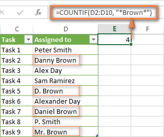
An asterisk (*) is used to find cells with any sequence of leading and trailing characters, as illustrated in the above example. If you need to match any single character, enter a question mark (?) instead, as demonstrated below.
Tip. It is also possible to use wildcards with cell references with the help of the concatenation operator (&). For example, instead of supplying "*Brown*" directly in the formula, you can type it in some cell, say F1, and use the following formula to count cells containing "Brown": =COUNTIF(D2:D10, "*"&F1&"*")
Count cells beginning or ending with certain characters
You can use either wildcard character, asterisk (*) or question mark (?), with the criterion depending on which exactly result you want to achieve.
If you want to know the number of cells that start or end with certain text no matter how many other characters a cell contains, use these formulas:
=COUNTIF(C2:C10,"Mr*") - count cells that begin with "Mr".
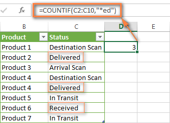
=COUNTIF(C2:C10,"*ed") - count cells that end with the letters "ed".
The image below demonstrates the second formula in action:
If you are looking for a count of cells that start or end with certain letters and contain the exact number of characters, you use the Excel COUNTIF function with the question mark character (?) in the criteria:
=COUNTIF(D2:D9,"??own") - counts the number of cells ending with the letters "own" and having exactly 5 characters in cells D2 through D9, including spaces.
=COUNTIF(D2:D9,"Mr??????") - counts the number of cells starting with the letters "Mr" and having exactly 8 characters in cells D2 through D9, including spaces.
Tip. To find the number of cells containing an actual question mark or asterisk, type a tilde (~) before the ? or * character in the formula. For example, =COUNTIF(D2:D9,"*~?*") will count all cells containing the question mark in the range D2:D9.
Excel COUNTIF for blank and non-blank cells
These formula examples demonstrate how you can use the COUNTIF function in Excel to count the number of empty or non-empty cells in a specified range.
COUNTIF not blank
In some Excel COUNTIF tutorials and other online resources, you may come across formulas for counting non-blank cells in Excel similar to this one:
=COUNTIF(A1:A10,"*")
But the fact is, the above formula counts only cells containing any text values including empty strings, meaning that cells with dates and numbers will be treated as blank cells and not included in the count!
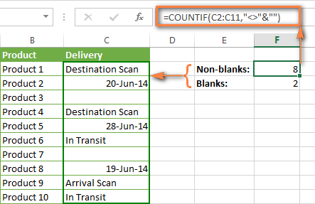
If you need a universal COUNTIF formula for counting all non-blank cells in a specified range, here you go:
Or
This formula works correctly with all value types - text, dates and numbers - as you can see in the screenshot below.
COUNTIF blank
If you want the opposite, i.e. count blank cells in a certain range, you should adhere to the same approach - use a formula with a wildcard character for text values and with the "" criteria to count all empty cells.
Formula to count cells not containing any text:
Since an asterisk (*) matches any sequence of text characters, the formula counts cells not equal to *, i.e. not containing any text in the specified range.
Universal COUNTIF formula for blanks (all value types):
The above formula correctly handles numbers, dates and text values. For example, here's how you can get the number of empty cells in the range C2:C11:
=COUNTIF(C2:C11,"")
Please be aware that Microsoft Excel has another function for counting blank cells, COUNTBLANK. For instance, the following formulas will produce exactly the same results as the COUNTIF formulas you see in the screenshot above:
Count blanks:
=COUNTBLANK(C2:C11)
Count non-blanks:
=ROWS(C2:C11)*COLUMNS(C2:C11)-COUNTBLANK(C2:C11)
Also, please keep in mind that both COUNTIF and COUNTBLANK count cells with empty strings that only look blank. If you do not want to treat such cells as blanks, use "=" for criteria. For example:
=COUNTIF(C2:C11,"=")
For more information about counting blanks and not blanks in Excel, please see:
COUNTIF greater than, less than or equal to
To count cells with values greater than, less than or equal to the number you specify, you simply add a corresponding operator to the criteria, as shown in the table below.
Please pay attention that in COUNTIF formulas, an operator with a number are always enclosed in quotes.
| Criteria | Formula Example | Description |
|---|---|---|
| Count if greater than | =COUNTIF(A2:A10,">5") | Count cells where value is greater than 5. |
| Count if less than | =COUNTIF(A2:A10,"<5") | Count cells with values less than 5. |
| Count if equal to | =COUNTIF(A2:A10,"=5") | Count cells where value is equal to 5. |
| Count if not equal to | =COUNTIF(A2:A10,"<>5") | Count cells where value is not equal to 5. |
| Count if greater than or equal to | =COUNTIF(C2:C8,">=5") | Count cells where value is greater than or equal to 5. |
| Count if less than or equal to | =COUNTIF(C2:C8,"<=5") | Count cells where value is less than or equal to 5. |
You can also use all of the above formulas to count cells based on another cell value, you will just need to replace the number in the criteria with a cell reference.
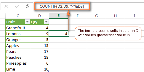
Note. In case of a cell reference, you have to enclose the operator in quotes and add an ampersand (&) before the cell reference. For example, to count cells in the range D2:D9 with values greater than a value in cell D3, you use this formula =COUNTIF(D2:D9,">"&D3):
If you want to count cells that contain an actual operator as part of the cell's contents, i.e. the characters ">", "<" or "=", then use a wildcard character with the operator in the criteria. Such criteria will be treated as a text string rather than a numeric expression. For example, the formula =COUNTIF(D2:D9,"*>5*") will count all cells in the range D2:D9 with contents like this "Delivery >5 days" or ">5 available".
Using Excel COUNTIF function with dates
If you want to count cells with dates that are greater than, less than or equal to the date you specify or date in another cell, you proceed in the already familiar way using formulas similar to the ones we discussed a moment ago. All of the above formulas work for dates as well as for numbers. Let me give you just a few examples:
| Criteria | Formula Example | Description |
|---|---|---|
| Count dates equal to the specified date. | =COUNTIF(B2:B10,"6/1/2014") | Counts the number of cells in the range B2:B10 with the date 1-Jun-2014. |
| Count dates greater than or equal to another date. | =COUNTIF(B2:B10,">=6/1/2014") | Count the number of cells in the range B2:B10 with a date greater than or equal to 6/1/2014. |
| Count dates greater than or equal to a date in another cell, minus x days. | =COUNTIF(B2:B10,">="&B2-"7") | Count the number of cells in the range B2:B10 with a date greater than or equal to the date in B2 minus 7 days. |
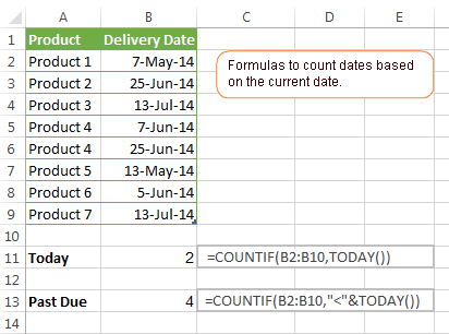
Apart from these common usages, you can utilize the COUNTIF function in conjunction with specific Excel Date and Time functions such as TODAY() to count cells based on the current date.
| Criteria | Formula Example |
|---|---|
| Count dates equal to the current date. | =COUNTIF(A2:A10,TODAY()) |
| Count dates prior to the current date, i.e. less than today. | =COUNTIF(A2:A10,"<"&TODAY()) |
| Count dates after the current date, i.e. greater than today. | =COUNTIF(A2:A10,">"&TODAY()) |
| Count dates that are due in a week. | =COUNTIF(A2:A10,"="&TODAY()+7) |
| Count dates in a specific date range. | =COUNTIF(B2:B10, ">=6/1/2014")-COUNTIF(B2:B10, ">6/7/2014") |
Here is an example of using such formulas on real data (at the moment of writing today was 25-Jun-2014):
Excel COUNTIF with multiple criteria
In fact, Excel COUNTIF function is not exactly designed to count cells with multiple criteria. In most cases, you'd use its plural counterpart, the COUNTIFS function to count cells that match two or more criteria (AND logic). However, some tasks can be solved by combining two or more COUNTIF functions in one formula.
Count values between two numbers
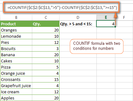
One of the most common applications of Excel COUNTIF function with 2 criteria is counting numbers within a specific range, i.e. less than X but greater than Y. For example, you can use the following formula to count cells in the range B2:B9 where a value is greater than 5 and less than 15.
=COUNTIF(B2:B9,">5")-COUNTIF(B2:B9,">=15")
How this formula works:
Here, we use two separate COUNTIF functions - the first one finds out how many values are greater than 5 and the other one gets a count of values greater than or equal to 15. Then, you subtract the latter from the former and get the desired result.
Count cells with multiple OR criteria
In situations when you want to get several different items in a range, add 2 or more COUNTIF functions together. Supposing, you have a shopping list and you want to find out how many soft drinks are included. To have it done, use a formula similar to this:
=COUNTIF(B2:B13,"Lemonade")+COUNTIF(B2:B13,"*juice")
Please pay attention that we've included the wildcard character (*) in the second criterion, it is used to count all kinds of juice on the list.
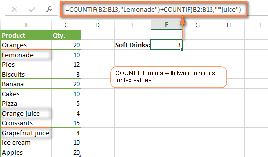
In the same manner, you can write a COUNTIF formula with several conditions. Here is an example of the COUNTIF formula with multiple OR conditions that counts lemonade, juice and ice cream:
=COUNTIF(B2:B13,"Lemonade") + COUNTIF(B2:B13,"*juice") + COUNTIF(B2:B13,"Ice cream")
For other ways to count cells with OR logic, please see this tutorial: Excel COUNTIF and COUNTIFS with OR conditions.
Using COUNTIF function to find duplicates and unique values
Another possible usage of the COUNTIF function in Excel is for finding duplicates in one column, between two columns, or in a row.
Example 1. Find and count duplicates in 1 column
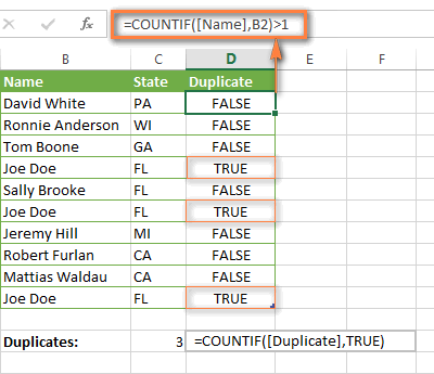
For example, this simple formula =COUNTIF(B2:B10,B2)>1 will spot all duplicate entries in the range B2:B10 while another function =COUNTIF(B2:B10,TRUE) will tell you how many dupes are there:
Example 2. Count duplicates between two columns
If you have two separate lists, say lists of names in columns B and C, and you want to know how many names appear in both columns, you can use Excel COUNTIF in combination with the SUMPRODUCT function to count duplicates:
=SUMPRODUCT((COUNTIF(B2:B1000,C2:C1000)>0)*(C2:C1000<>""))
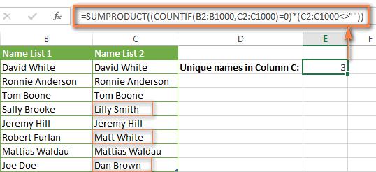
We can even take a step further and count how many unique names there are in Column C, i.e. names that do NOT appear in Column B:
=SUMPRODUCT((COUNTIF(B2:B1000,C2:C1000)=0)*(C2:C1000<>""))
Tip. If you want to highlight duplicate cells or entire rows containing duplicate entries, you can create conditional formatting rules based on the COUNTIF formulas, as demonstrated in this tutorial - Excel conditional formatting formulas to highlight duplicates.
Example 3. Count duplicates and unique values in a row
If you want to count duplicates or unique values in a certain row rather than a column, use one of the below formulas. These formulas might be helpful, say, to analyze the lottery draw history.
Count duplicates in a row:
=SUMPRODUCT((COUNTIF(A2:I2,A2:I2)>1)*(A2:I2<>""))
Count unique values in a row:
=SUMPRODUCT((COUNTIF(A2:I2,A2:I2)=1)*(A2:I2<>""))

Excel COUNTIF - frequently asked questions and issues
I hope these examples have helped you to get a feel for the Excel COUNTIF function. If you've tried any of the above formulas on your data and were not able to get them to work or are having a problem with the formula you created, please look through the following 5 most common issues. There is a good chance that you will find the answer or a helpful tip there.
1. COUNTIF on a non-contiguous range of cells
Question: How can I use COUNTIF in Excel on a non-contiguous range or a selection of cells?
Answer: Excel COUNTIF does not work on non-adjacent ranges, nor does its syntax allow specifying several individual cells as the first parameter. Instead, you can use a combination of several COUNTIF functions:
Wrong: =COUNTIF(A2,B3,C4,">0")
Right: =COUNTIF(A2,">0") + COUNTIF(B3,">0") + COUNTIF(C4,">0")
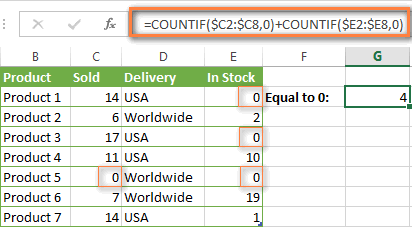
An alternative way is using the INDIRECT function to create an array of ranges. For example, both of the below formulas produce the same result you see in the screenshot:
=SUM(COUNTIF(INDIRECT({"B2:B8","D2:C8"}),"=0"))
=COUNTIF($B2:$B8,0) + COUNTIF($C2:$C8,0)
2. Ampersand and quotes in COUNTIF formulas
Question: When do I need to use an ampersand in a COUNTIF formula?
Answer: It is probably the trickiest part of the COUNTIF function, which I personally find very confusing. Though if you give it some thought, you'll see the reasoning behind it - an ampersand and quotes are needed to construct a text string for the argument. So, you can adhere to these rules:
If you use a number or a cell reference in the exact match criteria, you need neither ampersand nor quotes. For example:
=COUNTIF(A1:A10,10)
or
=COUNTIF(A1:A10,C1)
If your criteria includes text, wildcard character or logical operator with a number, enclose it in quotes. For example:
=COUNTIF(A2:A10,"lemons")
or
=COUNTIF(A2:A10,"*") or =COUNTIF(A2:A10,">5")
In case your criteria is an expression with a cell reference or another Excel function, you have to use the quotes ("") to start a text string and ampersand (&) to concatenate and finish the string off. For example:
=COUNTIF(A2:A10,">"&D2)
or
=COUNTIF(A2:A10,"<="&TODAY())
If you are in doubt whether an ampersand is needed or not, try out both ways. In most cases an ampersand works just fine, e.g. both of the below formulas work equally well.
=COUNTIF(C2:C8,"<=5")
and
=COUNTIF(C2:C8,"<="&5)
3. COUNTIF for formatted (color coded) cells
Question: How do I count cells by fill or font color rather than by values?
Answer: Regrettably, the syntax of the Excel COUNTIF function does not allow using formats as the condition. The only possible way to count or sum cells based on their color is using a macro, or more precisely an Excel User-Defined function. You can find the code working for cells colored manually as well as for conditionally formatted cells in this article - How to count and sum Excel cells by fill and font color.
4. #NAME? error in the COUNTIF formula
Issue: My COUNTIF formula throws a #NAME? error. How can I get it fixed?
Answer: Most likely, you have supplied an incorrect range to the formula. Please check out point 1 above.
5. Excel COUNTIF formula not working
Issue: My COUNTIF formula is not working! What have I done wrong?
Answer: If you have written a formula which is seemingly correct but it does not work or produces a wrong result, start by checking the most obvious things such as a range, conditions, cell references, use of ampersand and quotes.
Be very careful with using spaces in a COUNTIF formula. When creating one of the formulas for this article I was on the verge of pulling my hair out because the correct formula (I knew with certainty it was right!) wouldn't work. As it turned out, the problem was in a measly space somewhere in between, argh... For instance, look at this formula:
=COUNTIF(B2:B13," Lemonade").
At first sight, there is nothing wrong about it, except for an extra space after the opening quotation mark. Microsoft Excel will swallow the formula just fine without an error message, warning or any other indication, assuming you really want to count cells containing the word 'Lemonade' and a leading space.
If you use the COUNTIF function with multiple criteria, split the formula into several pieces and verify each function individually.
And this is all for today. In the next article, we will explore several ways to count cells in Excel with multiple conditions. Hope to see you next week and thanks for reading!
 by
by
1034 comments
Hi I have a question:
I have a list of values in Column A on tab 1 - Product
potato
tomato
squash
corn etc and they are unique
On the tab 2 I have 2 columns:
Column A has the same values as column A on tab 1 but they could repeat, and column B has some text, for example color. Not all column B is populated
potato brown
tomato red
potato purple
squash
corn yellow
I need to calc. value in col B on tab A, where it will count for each of the col A entries on tab A it will count how many have values on tab 2
So it will be on tab A
Potato 2
tomato 1
squash 0
corn 1
Thank you!
In column "S", I have numbers 1,2,3... (based on the formula that checks a value in Column A (if blank, gives blank... else a number in Ascending Order).
I have a similar value in Column X as well. 1,2,3,... etc.
in between, I have Certain values in Columns U & V (derived from certain formula). In column Y3 I am trying to calculate using the below formula...
=COUNTIFS(S:S,"<"&X3,V:V,U3)
but I am getting everything as '0'.
Please advice.
thanks,
Manish Gupta
=COUNTIF($D$9:$D$38,"B")+COUNTIF($J$9:$J$38,">=16")
with the above formula,I wanted to find out total numbers of boys passed and failed in three subjects,English,Maths,and science.Full mark is 40 and pass mark is 16
this is my table
sl Name gender english maths science
1 Sunny M 22 21 18
2 mike F 14 12 19
3 Bunny M 22 21 18
4 mike F 14 12 19
so I wanted to find out total boys and girls failed and passed using the formula
I have been reading up on this but have been unsuccessful in assembling a working formula to solve my issue.
I am downloading a YTD sales report weekly and need to report out some key KPI's.
The goal is to dump the sales report YTD extract into the model weekly and have all the KPI's update based on date ranges, dsum logic, etc.
I need to calculate the # of orders and the # of shipments (referencing a weekly date range).
The data from the extract has columns for order date, order #, item # and qty.
I need to calculate shipments, which would be the sum of all the unique order #'s for the date range (there are duplicated order #'s in the data extract).
I also need to calculate the # of orders by item. This is more tricky as there can be multiple lines for the same item on an order.
Please let me know if you have some suggestions for a simple formula based solution without sorting the data extract or using a pivot table.
Thanks in advance for any support.
B1 contains p.qdg2, p.qdg2xh
B2 contains p.qdg2x, p.qdg2
B3 contains p.qdg2xfe
B4 contains p.qdg2
Need to count number of times p.qdg2 occurs in range B1:B4
Only p.qdg2 should be counted - not p.qdg2x or p.qdg2xh or p.qdg2xfe
ie/ result should be 3
Can anyone can give me the formula please?
hi,
we have to required result how many R0715, R0716, R0718
R07150101
R07160110
R07150122
R07180129
R07150132
R07180137
R07170139
R07120147
R07150163
R07150168
R07150172
If your codes are in coloumn A...
=COUNTIF(A1:A12,"R0715*")
please help. how to make formula in numbering like this:
1. MMPSI16040052
1. MMPSI16040052
1. MMPSI16040052
2. MMPSI16040053
2. MMPSI16040053
3. MMPSI16040054
3. MMPSI16040054
Hi All,
Can I count a value that exists in columns rather than cells? For example, I want to know how many columns contain the number say 3, even if a single column has more than once cells that contains "3". I am interested in knowing the number of columns not how many times number "3" exists
Thanks in advance!
I would start by setting up a helper column containing an IF formula wrapped around a COUNTIF, for each column you are searching. For example, if columns A-F are the ones you are searching, then use G-L for these formulas. Each IF formula is to convert the results of a COUNTIF, into a 0 or 1, indicating whether that column contains that value.
Then in column M, use a SUM function to add up the results from the Helper columns G-L.
Below is the formula,
=COUNTIF(A1:Z100,3)
Change the range of the cells as required.
Vijaykumar Shetye, Goa, India
I inserted a wrong formula, sorry. Here it is what I tried.
=COUNTIFS(
Sheet1!$E$2:$E$5000;">="&A2;
Sheet1!$E$2:$E$5000;"<"&A3;
Sheet1!$B$2:$B$5000;"C"
)
Hello,
this makes me really crazy.
I have 3 different values in a column B and a timestamp in a column E. I have to create a graph with daily sum of values. (Line chart for A, B, C,...)
Sheet 1
========
A;2016.01.26. 15:55
A;2016.01.26. 18:11
A;2016.01.26. 21:10
A;2016.01.27.,01:02 --> extra comma here
B;2016.01.27. 10:10
B;2016.01.27. 10:01
C;27/01/2016 11:55 --> other time format
A;2016.01.28. 11:50
C;2016.01.28. 11:04
C;Fr 2016.01.28. 12:22 --> extra day field
B;2016.01.28. 12:09
A;2016.01.28. 13:31
I have thousands of records and well, some times the timestamp field has another format or has some error. :/
Sheet 2
========
Column A contains the date values (for the graph).
A2 = 2016.01.01
A3 = 2016.01.02
.
.
.
A32 = 2016.01.31
I tried this formula, not worked.
B2: =COUNTIFS(Sheet1!$E$2:$E$5000;">="&A2;Sheet1!$E$2:$E$5000;"="&A2;Sheet1!$E$2:$E$5000;"="&A2;Sheet1!$E$2:$E$5000;"<"&A3;Sheet1!$B$2:$B$5000;"C")
So, the result matrix should be like this:
2016.01.01; count-of-A-on-0101; count-of-B-on-0101; count-of-C-on-0101;
2016.01.01; count-of-A-on-0102; count-of-B-on-0102; count-of-C-on-0102;
2016.01.01; count-of-A-on-0103; count-of-B-on-0103; count-of-C-on-0103;
.
.
.
2016.01.31; count-of-A-on-0131; count-of-B-on-0131; count-of-C-on-0131;
I tried also name the ranges because I'd like to use the autofill function with the date parameters as running values.
Cheers:
Poljakov
Hi
Value in cell A3 is 10
I want to check this value tn 4 Different Criteria
1)Less than 20
2)Greater than 20 but less than 50
3)Greater than 50 but less than 80
4)greater than 80
Please help
Regards
Venkat
Hi Venkat,
Can you give more details on what you want to do? It looks like you have just 1 cell with a value but multiple mutually-exclusive criteria (10 cannot be less than 20 and also greater than 20). You may want multiple cells that use the COUNTIF function, or if you want to test the same cell for multiple criteria, use COUNTIFS.
Hope that helps!
Hello all,
I'm trying to build a dynamic graph where the x-axis and the data graphed are based on which checkboxes (January 2015, February 2015, ..., December 2016) are checked off. If the first checked checkbox is April 2015, I want that to be the first value on the x-axis. Similarly, if October 2016 is the last checked checkbox, I want the graph to end there.
To accomplish this, I have a table with True/False cells linked to each checkbox. If the checkbox is checked, then the corresponding cell value is TRUE and the cell next to that reads "January 2015" or whatever the corresponding month is.
If the checkbox is NOT checked, the value is FALSE and the cell next to that is "". I then created a named formula of "Months" that I have defined as =OFFSET(E3:E1000,0,0,COUNTA(E3:E1000),1).
However, this is counting all the cells with "" in them as not blank, and therefore is graphing all the months (i.e. x-axis is static). How can I define Months as only being the months that are checked off and not also the cells with "" in them?
Thank you!
i mean di ko po alam formula sa lahat na may #name?..
Sales Representative Month Amount
Jones Jan 20,000.00
Jones Jan 22,500.00
Rogers Jan 40,000.00
Rogers Mar 15,000.00
Rogers Jan 25,000.00
Franklin Apr 80,000.00
Franklin Feb 20,000.00
Jones Feb 35,000.00
Franklin Jan 12,000.00
Rogers Feb 90,000.00
Franklin Feb 75,000.00
Jones Feb 80,000.00
Total Sales for January 119,500.00
Total Sales for February 300,000.00
Total Sales of Jones 157,500.00
Total Sales of Franklin 187,000.00
Total Sales of Jones in January only #NAME?
Total Sales of Jones in February only #NAME?
Total Sales of Roger greater than 10000 #NAME?
Count Sales greater than 20000 8
Average sales of all agents in January #NAME?
itong my name po, pwede malaman kung ano formula nito?
Hi friends i need how to count the status,
Eg: Category A Category B
AAA Progress
AAA Quoted
AAA Quoted
BBB Awarded
CCC Quoted
I need AAA how many numbers Quoted respectively...
I want to count total of student in a certain month , for example: April 2015
I used =COUNTIF(A3:A4006,"April 2015") and I got zero.
it works but I think I missed something. Could you tell me?
Hi, I have a spreadsheet that is asking me to add a total of car rentals, there is a yes and no categoery going down to show if the customer is filling the car $65 so I need a function that will sub just the totals for the cust. that have n's and then sub + the $65 for only the cust with the y' here is an example.
A B C D E F
Date Dys rented Dly.rate T.bfore gas option Total
gs option
1 3 49.99 3x49.99 n(no +$65)
2 1 53.00 2x 53.00 y(+$65)
3 2 75.00 2x75.00 y (+65)
on A9 it says $65 , so A9 needs to go in the func and added to the y's for a grand total.but not added to the n's. Please help me with this function! The function needs to be in F1 and then I will copy the function down to the rest.
Hi,
How to link Hlook up data value with vlookup on a excel workbook between two spreadsheets . if i change a value in Hlookup Sheet it might be automatically change in v lookup sheet .your spurt is required . Thanks in Advance .
I am trying to count the number of cells in column j that is between 0 and 91, and that falls between a certain date (ie:4/30/2016)with the dates being in column L
example: How many people have worked less than 90 days during a particular month.
How to calculate number of similar value count as 1 by using countifs formula.
Can you tell what is wrong with COUNT formula? =COUNT(C5:C105,A4)
I have a PROBLEM which i face to maintain my stock.
I have some data in shhet1:
A B
S/L PRODUCT
1 CLR 0 R MER 5 R ZU 3 R
2 FYD 2 R DSR 3 R CLR 0 R
4 PML 3 R FGH 4 R LKN 0 R
5 DSR 4 R LKN 2 R ZU 1 R
NOW IN Sheet2
A B C
PRODUCT CODE
CLIARWAY CLR
BAG DSR
SPOON PML
JUG LKN PROBLEM IS I WANT TO COUNT AND ADD SHHEET 1 PRODUCT QUANTITY IN SHEET2 C CLOUMN E.G.
A B C
BAG DSR 7......IS IT POSSIBLE? PLEASE HELP ME THANK YOU.
Good Afternoon - I am attempting to count how many non-errors (#N/A) are in a VLookup column. For example, I might have a column of 500 errors, and 3 returned items. I need to know how to count those that are not returned as errors but as values. I can't seem to find a way to make this return back to me. Any help would be appreciated.
Hi madam,
iam struck with one error problem in excel.
There is list of students name in columnA : A1:A10
and also more students name in ColumnE : E1:E10
Now i want to count, how many times each name is repeated in both columns A and E using countif function.
Between A and E we have B, C,D columns contains different data columns.
COUNTIF(range, criteria)
i am not able to add both range under single criteria in countif function.
Please help me with the solution.
How to add two non adjacent column under single criteria.
=COUNTIF( both range?, "ravi")
A B C D E
1 ravi 435 Teja
2 sneha 250 sunil
3 anil 136 ravi
4 teja 786 sandy
5 sunil 250 praveen
6 reena 587 teena
7 naveen 121 praveen
8 sunil 456 anitha
9 teena 454 reena
10 sunil 895 anil
Hello, Praveen,
Here you are:
=COUNTIF(A1:A10, "ravi") + COUNTIF(E1:E10, "ravi")
can it possible to put both ranges A1:A10 and E1:E10 in single array like { A1:A10 E1:E10 } to reduce the formula length.
Hi bro(s),
I have a question about using COUNTIFS to count number of rows that have status different from "completed" with the example below:
Status-------Value
completed 1
started 2
canceled 3
delayed 5
Result expectation: 3
How can I count with the exactly string excluded? Please help me answer, I need your help!
Many thanks,
Ngan Trinh
Hello, Ngan,
Please try the formula below:
=COUNTIF(A2:A5,"<>"&"completed")
here the Status column is in A1:A5
I want to SUM up a row but the total has to be either a sum up or blank if there is an empty value (a blank cell).
i.e.
A B C D(A1+B1+C1)
1 12 28 30 70
2 50 20 17 87
3 10 34 06 50
4 "Blank"
5 20 20
I've tried
=COUNTIF(G17,">0")+COUNTIF(H17,">0")+COUNTIF(I17,">0")
also
=SUM(IF(ISBLANK(G17),IF(ISBLANK(H17),IF(ISBLANK(I17),G17+H17+I17,""))))
as well as
=SUM(IF(G17:I17"",G17:I17,""))
The answer of total still wrong.
How should I set the formula at D?
Thanks.
Hello, Peggie,
Please try this one:
=IF(OR(ISBLANK(A1), ISBLANK(B1), ISBLANK(C1)), "Blank", SUM(A1:C1))
I want to eliminate duplicate values and I have a problem with count if function, it gives error message even though i entered correct formula.
The formula i entered in data validation
=COUNTIF($E$2:$E$100,E2)=1
can you suggest possible solutions for getting error while using this formula.
Thanks
I am able to count using countif to get response to a particular column inmy worksheet, e.g, i could write countif(d12..d80,"Pass"). I want to add to this same expression to be able to look at another column, e.g., F and only count Pass where the corresponding number in a new cellF is equal to 10 or any number. How do I add this to the count if expression?
Thanks
I have a column of UPS, FedEx, and DHL tracking numbers. I am trying to sum up the total # of tracking numbers in that column. How can I do this when the tracking number has both text and number context in it?
e.g.:
36006962160000026558847083172014
1Z9V14091300013079
7614784914
Have you tried using the following code?:
=COUNTA(A1:A3)
Hi Svetlana
Following on from post 213, I have modified the formula slightly and used it as part of conditional formatting via the "Formula is" new rule and it works perfectly. Is there any way that the identified duplicate rows that meet the formula can be copied to a new sheet next available row? The formula is = AND(ISNUMBER(A1), ISNUMBER(B1), C1="", D1="",COUNTIF(E:E, E1)>1) any help or direction would be much appreciated.
I'm trying to calculate only the number of cells in which the employees start date is less than 90 from there last day worked. These dates are captured on two separate columns for multiple employees. I can't seem to figure this one out.
Your help is greatly appreciated.
I have the following data:
Case Rate
A 0
A 2.58
B 0
B 0
C 13.45
C 0
C 0
D 0
D 0
D 0
I need to determine how many of the case groups have a total of Zero. In the above example, it should read 2 case (Case B & D) arethe only one that has a zero total
Note - the case letters are only for this example, usually it will be different names
I have tried the following formula but it doesn't produce the results that I am looking for: =COUNTIFS(A2:A16,A2:A16,B2:B16,0)
Thanks a million, answered all the questions that Excel-help couldn't give me (particularly on how to count dates separately from text).
Keep it up!
Example 1. Find and count duplicates in 1 column
For example, this simple formula =COUNTIF(B2:B10,B2)>1 will spot all duplicate entries in the range B2:B10 while another function =COUNTIF(B2:B10,TRUE) will tell you how many dupes are there:
Good Day!
May I know what is the function of "B2" in this example >> =COUNTIF(B2:B10,B2)>1 ?
Thanks a zillion!
Hi, I want to count all cells that have numbers only. I have some cells that have NA and I want to exclude those from the calculation.
thanks,
Di
Hello, Di,
Please use the count() function.
Help needed... I am trying to read number of cells which match "check" in another excel document and count if formula is not working correctly.I have a document "X1" at "C:\Users\XY123\Documents\Work\" which I named as sheet1_XLSX(C:\Users\XY123\Documents\Work\X1.xlsx). I am using this formula to open and do countif function like this : =Countif('[sheet1_xlsx]sheet1_xlsx.xlsx'!$E:$E,"check"). But the formula is returning as #value!.
hi Svetlana, i have created an any year calendar and i want to mention holidays, here in Sri Lanka, the holiday will differ every year, so how i can display holiday by manual for every year?
Thawfeeque.
Hi Svetlana, I'm trying to identify duplicates in a column based on values in adjacent cells. For example:
A B C D E
375 500 Cheddar (D)
Soft Brie
125 Hard Cheddar
125 375 Cheddar (D)
375 Soft Brie
A & B are number format; C, D and E are Text format.
For a duplicate to be correct A & B must have numbers present, C & D must be blank - I have indicated the duplicates here with a (D) but not needed in the formula. If I had hair I would have lost it today trying to figure this out - please help.
Hi Roy,
If my understanding of the task is correct, the following formula should work a treat:
=IF(AND(ISNUMBER(A1), ISNUMBER(B1), C1="", D1=""), IF(COUNTIF(E:E, E1)>1, "dupe", ""), "")
REF: 213
Hi Svetlana many thanks for the quick reply. I was just venturing in to the ISNUMBER function when your solution arrived. Yes it works thank you, however, it doesn't wait for a comparison before stating "dupe" - my fault for not being very clear. Unless I'm mistaken ISNUMBER only caters for a single cell and not a range - is there a way around this please?
Hi Roy,
Yes, ISNUMBER accepts only an individual cell in the argument. Sorry, I do not quite understand what you mean when saying "it doesn't wait for a comparison before stating "dupe". Please specify what cells should be compared.
The formula I suggested works with the following logic:
If A1 & B1 have any numbers in them, and C1 & D1 are blank, check column E for duplicate values (i.e. check if the value in E1 occurs in any other cell in column E). If one or more duplicates are found, the formula returns "dupe", an empty string otherwise.
Hi Svetlana
Essentially, when I re-read what I have asked of you, you have responded by producing exactly what I requested - my apologies for the lack of clarity. To keep it its simplest terms, I have a range of cells A1:E20 where a duplicate condition is met when a row has A1 & B1 with numbers in them and both C1 & D1 are blank, E1 would then be checked for duplicate values. However, on the first occasion that this occurs it cannot be considered a duplicate it is a unique value until a second occurrence appears etc. I have been trying COUNTA in place of ISNUMBER, still not quite there but I think it's the last bit that might be the key.
Once again apologies for the confusion, I really appreciate what you and the team at Ablebits do in supporting us lesser mortals.
Hi Roy,
No need to apologize. From my own experience, it's very difficult to exactly explain/understand the task without seeing the same source data :)
Please try the following formula. It identifies duplicates without 1st occurrences:
=IF(AND(ISNUMBER(A1), ISNUMBER(B1), C1="", D1=""), IF(COUNTIF($E$1:$E1, $E1)>1, "dupe", ""), "")
Is this what you are looking for?
Yes Svetlana - works a treat - great job - have a good weekend!
I have a worksheet that contains all my sales of various products to various customers over several weeks.
Assuming column B lists the customers, column c lists the products, and columns f to z lists the sales volume sold each week, how can I determine the number of unique customers (col b) that purchased at least 1 of any product in any given week (col f to z)... given that customers could purchase multiple products in any week and be listed multiple times in col b?
Thanks
Hi Please im begging for your help on this please.
i have a problem with countif. how will i count Arriola with more than 2 days? i dont want to count arriola i want to count only arriola with more than 2 days.. please
A B MORE THAN 2 days
Lionel 2 Lionel = 0 << LIKE THIS RESULT
Lionel 2 Arriola = 1
Arriola 3
Arriola 1
Lionel 2
Arriola 2
Hi!
To count cells with 2 or more criteria, you need to use the COUNTIFS function.
Supposing that "Arriola" is in column and the number of days in column B, you can use the following formula:
=COUNTIFS(A:A, "Arriola", B:B, ">2")
A B
1 Grn:1 11-01-2016
2 Grn:2 11-01-2016
3 Grn:2 11-01-2016
4 Grn:3 11-01-2016
in this table i want to count in 11-Jan-16 how many GRN I received it should not count double like GRN:2 i received 2 time in same date so i want to count only one time.
Hello Sunil,
I recommend adding a column that will check if the values have duplicates. Then you can use the COUNTIFS function to calculate the result by two criteria.
https://www.ablebits.com/office-addins-blog/excel-countifs-multiple-criteria/
Please see a sample file with the functions that I described:
https://support.ablebits.com/blog_samples/excel-countif-examples_210.xlsx
Our Excel add-in that allows to remove duplicate rows can also be helpful for you:
https://www.ablebits.com/excel-suite/find-remove-duplicates.php
I am having one doubt regarding counting value like
A B
1 Grn:1 11-01-2016 in this table i want to count in 11-Jan-16 how
2 Grn:2 11-01-2016 many GRN I received it should not count double
3 Grn:2 11-01-2016 like GRN:2 i received 2 time in same date so i
4 Grn:3 11-01-2016 want to count only one time.
Please help
Hello Sunil,
Please see a sample file and my next answer:
https://support.ablebits.com/blog_samples/excel-countif-examples_210.xlsx
Hi Svetlana,
I am trying to calculate the number of countries with a life expectancy between 50-55,55-60,60-65...etc.
columnA: country name
ColumnB: Average life exp.
would i be able to use the =countif function to find he amount of countries with the given criteria?
Hi Noah,
To count with multiple criteria, you need to use the COUNTIFS fucntion. For example:
=COUNTIFS(B:B, ">=50", B:B, "<=55")
So how do you drag it down to reflect the count of the changing range without manipulating the individual cells manually.
For eg. 50-65
And next cell will be 70-75, etc
Hello Svetlana
I have a spreadsheet where i have to count the amount of unique rows in column C that had the value "UDL" in column N.
Column C can have duplicates so somehow i need to find out how many unique ones there are
Hello Peter,
You need the following array formula (remember to press Ctrl + Shift + Enter to complete it):
=SUM(IF( (--($N1:$N31="UDL"))*(--(COUNTIF($C$1:$C$31,$C1:$C31)=1)),1,0))
With row 1 being the first, and row 31 being the last.
Uniques imply that there is only one occurrence of the value in column C.
If you need unique values plus the first occurrences of the duplicates, then you need to use a Helper column, e.g. column O, and enter the following formula into its first cell:
=IF(COUNTIF($C$1:$C1,$C1)=1,"Unique","Duplicate")
Paste the formula to all cells below.
Then use the following formula to count:
=COUNTIFS(N1:N31,"UDL",O1:O31,"Unique")
You can also use the Helper column to count only uniques, then the initial formula should look the following way:
=IF(COUNTIF($C$1:$C$31,$C1)=1,"Unique","Duplicate")
Sorry for question.
found answer as COUNTIFS(A1:A1001,1,B2:B1002,2).
Thank you anyway.
i have columns of headings standard MHRs and Actual MHRs I want to count the values in columns heading std mhrs.
Hi,
I wonder can you help,please
When I use COUNTIFS(A:A,A7,B:B,B2) this reads as doubles on same line no matter what the starting numbers.I use this in Lotto results and would like it to read from two different results,in stepwise format A:A,A1,B:B,B2,or is there a better way to do this,thank you in advance.
A B
1 Product Loan Range
2 Salary Loan <250
3 Salary Loan <250
4 Home Mortgage 250 < 350
Now i want to count how many salary loan under "<250"
=COUNTIFS(A2:A4,"Salary Loan",B2:B4,"<250")
Here am getting answer is zero. Since it is counting less than 250. But the Salary Loan under loan range "<250" counts 2 times.
I solved this issue by converting Range B to value 250,250-350,..
Is there any way to count without changing the format in Range B.
Hello
I have a question regarding a spreadsheet I am putting together and I am unsure if using counts would be the best way.
ITEM # | TRANS CODE | DOC DATE
AA R 10/1/15
AA R 10/1/15
AA R 10/2/15
AB R 10/1/15
AB R 10/1/15
AC R 10/2/15
In the above example I have three part numbers, AA, AB, and AC. Each one is a receipt on the day in the last column.
I am trying to count the number of receipt days in a week for each part, not just the number of receipts per day.
So for the AA I would have two receipt days (10/1 and 10/2), for the AB and the AC I would have one receipt day.
If I were counting the number of receipts would results in AA:3,AB:2,AC:1
My problem is I can not figure out how to do the code so that way when I type in the part number it returns and then sums the number of receipt days and not the number of receipts.
Hello Jess,
I recommend adding a column that will check if the values have duplicates
=IF(COUNTIF(B6:$B$11,B6)=1,"no duplicate","has duplicate below").
Then you can use a Pivot Table to count filtered values.
Please see a sample file with the functions that I described:
https://support.ablebits.com/blog_samples/excel-countif-examples_202.xlsx
Our Excel add-in that allows to remove duplicate rows can also be helpful for you:
https://www.ablebits.com/excel-suite/find-remove-duplicates.php
Hello,
Example: =COUNTIF('C:\Users\Desktop\[test.xlsx]List1'!$B$1:$B$10;B11)
Why when I close test.xlsx file this function returns #Value!# error?
(for other functions a link is not problem)
thank you for your answer, really :)
Hello Lukas,
Unfortunately I haven't found a way to get the formula re-calculated correctly without an open book.