Microsoft Excel provides several functions purposed for counting different kinds of cells, such as blanks or non-blanks, with number, date or text values, containing specific words or character, etc.
In this article, we will focus on the Excel COUNTIF function that is purposed for counting cells with the condition you specify. First, we will briefly cover the syntax and general usage, and then I provide a number of examples and warn about possible quirks when using this function with multiple criteria and specific types of cells.
In essence, COUNTIF formulas are identical in all Excel versions, so you can use the examples from this tutorial in Excel 365, 2021, 2019, 2016, 2013, 2010 and 2007.
COUNTIF function in Excel - syntax and usage
Excel COUNTIF function is used for counting cells within a specified range that meet a certain criterion, or condition.
For example, you can write a COUNTIF formula to find out how many cells in your worksheet contain a number greater than or less than the number you specify. Another typical use of COUNTIF in Excel is for counting cells with a specific word or starting with a particular letter(s).
The syntax of the COUNTIF function is very simple:
As you see, there are only 2 arguments, both of which are required:
- range - defines one or several cells to count. You put the range in a formula like you usually do in Excel, e.g. A1:A20.
- criteria - defines the condition that tells the function which cells to count. It can be a number, text string, cell reference or expression. For instance, you can use the criteria like these: "10", A2, ">=10", "some text".
And here is the simplest example of Excel COUNTIF function. What you see in the image below is the list of the best tennis players for the last 14 years. The formula =COUNTIF(C2:C15,"Roger Federer") counts how many times Roger Federer's name is on the list:
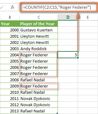
Note. A criterion is case insensitive, meaning that if you type "roger federer" as the criteria in the above formula, this will produce the same result.
Excel COUNTIF function examples
As you have just seen, the syntax of the COUNTIF function is very simple. However, it allows for many possible variations of the criteria, including wildcard characters, the values of other cells, and even other Excel functions. This diversity makes the COUNTIF function really powerful and fit for many tasks, as you will see in the examples that follow.
COUNTIF formula for text and numbers (exact match)
In fact, we discussed the COUNTIF function that counts text values matching a specified criterion exactly a moment ago. Let me remind you that formula for cells containing an exact string of text: =COUNTIF(C2:C15,"Roger Federer"). So, you enter:
- A range as the first parameter;
- A comma as the delimiter;
- A word or several words enclosed in quotes as the criteria.
Instead of typing text, you can use a reference to any cell containing that word or words and get absolutely the same results, e.g. =COUNTIF(C1:C9,C7).
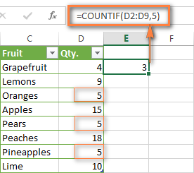
Similarly, COUNTIF formulas work for numbers. As shown in the screenshot below, the below formula perfectly counts cells with quantity 5 in Column D:
=COUNTIF(D2:D9, 5)
In this article, you will find a few more formulas to count cells that contain any text, specific characters or only filtered cells.
COUNTIF formulas with wildcard characters (partial match)
In case your Excel data include several variations of the keyword(s) you want to count, then you can use a wildcard character to count all the cells containing a certain word, phrase or letters as part of the cell's contents.
Suppose, you have a list of tasks assigned to different persons, and you want to know the number of tasks assigned to Danny Brown. Because Danny's name is written in several different ways, we enter "*Brown*" as the search criteria =COUNTIF(D2:D10, "*Brown*").
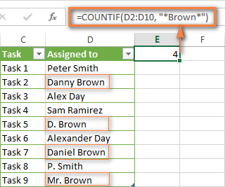
An asterisk (*) is used to find cells with any sequence of leading and trailing characters, as illustrated in the above example. If you need to match any single character, enter a question mark (?) instead, as demonstrated below.
Tip. It is also possible to use wildcards with cell references with the help of the concatenation operator (&). For example, instead of supplying "*Brown*" directly in the formula, you can type it in some cell, say F1, and use the following formula to count cells containing "Brown": =COUNTIF(D2:D10, "*"&F1&"*")
Count cells beginning or ending with certain characters
You can use either wildcard character, asterisk (*) or question mark (?), with the criterion depending on which exactly result you want to achieve.
If you want to know the number of cells that start or end with certain text no matter how many other characters a cell contains, use these formulas:
=COUNTIF(C2:C10,"Mr*") - count cells that begin with "Mr".
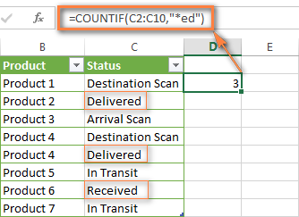
=COUNTIF(C2:C10,"*ed") - count cells that end with the letters "ed".
The image below demonstrates the second formula in action:
If you are looking for a count of cells that start or end with certain letters and contain the exact number of characters, you use the Excel COUNTIF function with the question mark character (?) in the criteria:
=COUNTIF(D2:D9,"??own") - counts the number of cells ending with the letters "own" and having exactly 5 characters in cells D2 through D9, including spaces.
=COUNTIF(D2:D9,"Mr??????") - counts the number of cells starting with the letters "Mr" and having exactly 8 characters in cells D2 through D9, including spaces.
Tip. To find the number of cells containing an actual question mark or asterisk, type a tilde (~) before the ? or * character in the formula. For example, =COUNTIF(D2:D9,"*~?*") will count all cells containing the question mark in the range D2:D9.
Excel COUNTIF for blank and non-blank cells
These formula examples demonstrate how you can use the COUNTIF function in Excel to count the number of empty or non-empty cells in a specified range.
COUNTIF not blank
In some Excel COUNTIF tutorials and other online resources, you may come across formulas for counting non-blank cells in Excel similar to this one:
=COUNTIF(A1:A10,"*")
But the fact is, the above formula counts only cells containing any text values including empty strings, meaning that cells with dates and numbers will be treated as blank cells and not included in the count!
If you need a universal COUNTIF formula for counting all non-blank cells in a specified range, here you go:
Or
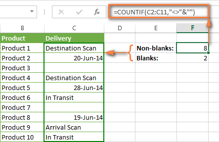
This formula works correctly with all value types - text, dates and numbers - as you can see in the screenshot below.
COUNTIF blank
If you want the opposite, i.e. count blank cells in a certain range, you should adhere to the same approach - use a formula with a wildcard character for text values and with the "" criteria to count all empty cells.
Formula to count cells not containing any text:
Since an asterisk (*) matches any sequence of text characters, the formula counts cells not equal to *, i.e. not containing any text in the specified range.
Universal COUNTIF formula for blanks (all value types):
The above formula correctly handles numbers, dates and text values. For example, here's how you can get the number of empty cells in the range C2:C11:
=COUNTIF(C2:C11,"")
Please be aware that Microsoft Excel has another function for counting blank cells, COUNTBLANK. For instance, the following formulas will produce exactly the same results as the COUNTIF formulas you see in the screenshot above:
Count blanks:
=COUNTBLANK(C2:C11)
Count non-blanks:
=ROWS(C2:C11)*COLUMNS(C2:C11)-COUNTBLANK(C2:C11)
Also, please keep in mind that both COUNTIF and COUNTBLANK count cells with empty strings that only look blank. If you do not want to treat such cells as blanks, use "=" for criteria. For example:
=COUNTIF(C2:C11,"=")
For more information about counting blanks and not blanks in Excel, please see:
COUNTIF greater than, less than or equal to
To count cells with values greater than, less than or equal to the number you specify, you simply add a corresponding operator to the criteria, as shown in the table below.
Please pay attention that in COUNTIF formulas, an operator with a number are always enclosed in quotes.
| Criteria | Formula Example | Description |
|---|---|---|
| Count if greater than | =COUNTIF(A2:A10,">5") | Count cells where value is greater than 5. |
| Count if less than | =COUNTIF(A2:A10,"<5") | Count cells with values less than 5. |
| Count if equal to | =COUNTIF(A2:A10,"=5") | Count cells where value is equal to 5. |
| Count if not equal to | =COUNTIF(A2:A10,"<>5") | Count cells where value is not equal to 5. |
| Count if greater than or equal to | =COUNTIF(C2:C8,">=5") | Count cells where value is greater than or equal to 5. |
| Count if less than or equal to | =COUNTIF(C2:C8,"<=5") | Count cells where value is less than or equal to 5. |
You can also use all of the above formulas to count cells based on another cell value, you will just need to replace the number in the criteria with a cell reference.
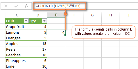
Note. In case of a cell reference, you have to enclose the operator in quotes and add an ampersand (&) before the cell reference. For example, to count cells in the range D2:D9 with values greater than a value in cell D3, you use this formula =COUNTIF(D2:D9,">"&D3):
If you want to count cells that contain an actual operator as part of the cell's contents, i.e. the characters ">", "<" or "=", then use a wildcard character with the operator in the criteria. Such criteria will be treated as a text string rather than a numeric expression. For example, the formula =COUNTIF(D2:D9,"*>5*") will count all cells in the range D2:D9 with contents like this "Delivery >5 days" or ">5 available".
Using Excel COUNTIF function with dates
If you want to count cells with dates that are greater than, less than or equal to the date you specify or date in another cell, you proceed in the already familiar way using formulas similar to the ones we discussed a moment ago. All of the above formulas work for dates as well as for numbers. Let me give you just a few examples:
| Criteria | Formula Example | Description |
|---|---|---|
| Count dates equal to the specified date. | =COUNTIF(B2:B10,"6/1/2014") | Counts the number of cells in the range B2:B10 with the date 1-Jun-2014. |
| Count dates greater than or equal to another date. | =COUNTIF(B2:B10,">=6/1/2014") | Count the number of cells in the range B2:B10 with a date greater than or equal to 6/1/2014. |
| Count dates greater than or equal to a date in another cell, minus x days. | =COUNTIF(B2:B10,">="&B2-"7") | Count the number of cells in the range B2:B10 with a date greater than or equal to the date in B2 minus 7 days. |
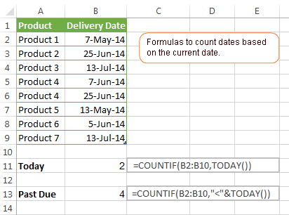
Apart from these common usages, you can utilize the COUNTIF function in conjunction with specific Excel Date and Time functions such as TODAY() to count cells based on the current date.
| Criteria | Formula Example |
|---|---|
| Count dates equal to the current date. | =COUNTIF(A2:A10,TODAY()) |
| Count dates prior to the current date, i.e. less than today. | =COUNTIF(A2:A10,"<"&TODAY()) |
| Count dates after the current date, i.e. greater than today. | =COUNTIF(A2:A10,">"&TODAY()) |
| Count dates that are due in a week. | =COUNTIF(A2:A10,"="&TODAY()+7) |
| Count dates in a specific date range. | =COUNTIF(B2:B10, ">=6/1/2014")-COUNTIF(B2:B10, ">6/7/2014") |
Here is an example of using such formulas on real data (at the moment of writing today was 25-Jun-2014):
Excel COUNTIF with multiple criteria
In fact, Excel COUNTIF function is not exactly designed to count cells with multiple criteria. In most cases, you'd use its plural counterpart, the COUNTIFS function to count cells that match two or more criteria (AND logic). However, some tasks can be solved by combining two or more COUNTIF functions in one formula.
Count values between two numbers
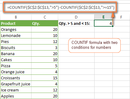
One of the most common applications of Excel COUNTIF function with 2 criteria is counting numbers within a specific range, i.e. less than X but greater than Y. For example, you can use the following formula to count cells in the range B2:B9 where a value is greater than 5 and less than 15.
=COUNTIF(B2:B9,">5")-COUNTIF(B2:B9,">=15")
How this formula works:
Here, we use two separate COUNTIF functions - the first one finds out how many values are greater than 5 and the other one gets a count of values greater than or equal to 15. Then, you subtract the latter from the former and get the desired result.
Count cells with multiple OR criteria
In situations when you want to get several different items in a range, add 2 or more COUNTIF functions together. Supposing, you have a shopping list and you want to find out how many soft drinks are included. To have it done, use a formula similar to this:
=COUNTIF(B2:B13,"Lemonade")+COUNTIF(B2:B13,"*juice")
Please pay attention that we've included the wildcard character (*) in the second criterion, it is used to count all kinds of juice on the list.
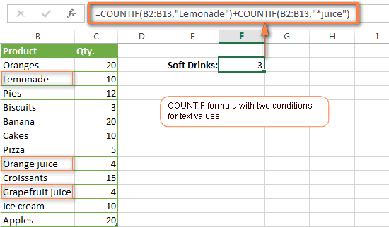
In the same manner, you can write a COUNTIF formula with several conditions. Here is an example of the COUNTIF formula with multiple OR conditions that counts lemonade, juice and ice cream:
=COUNTIF(B2:B13,"Lemonade") + COUNTIF(B2:B13,"*juice") + COUNTIF(B2:B13,"Ice cream")
For other ways to count cells with OR logic, please see this tutorial: Excel COUNTIF and COUNTIFS with OR conditions.
Using COUNTIF function to find duplicates and unique values
Another possible usage of the COUNTIF function in Excel is for finding duplicates in one column, between two columns, or in a row.
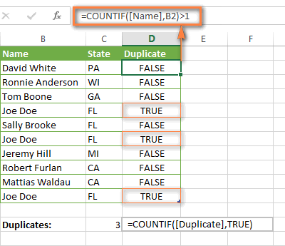
Example 1. Find and count duplicates in 1 column
For example, this simple formula =COUNTIF(B2:B10,B2)>1 will spot all duplicate entries in the range B2:B10 while another function =COUNTIF(B2:B10,TRUE) will tell you how many dupes are there:
Example 2. Count duplicates between two columns
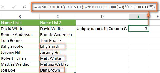
If you have two separate lists, say lists of names in columns B and C, and you want to know how many names appear in both columns, you can use Excel COUNTIF in combination with the SUMPRODUCT function to count duplicates:
=SUMPRODUCT((COUNTIF(B2:B1000,C2:C1000)>0)*(C2:C1000<>""))
We can even take a step further and count how many unique names there are in Column C, i.e. names that do NOT appear in Column B:
=SUMPRODUCT((COUNTIF(B2:B1000,C2:C1000)=0)*(C2:C1000<>""))
Tip. If you want to highlight duplicate cells or entire rows containing duplicate entries, you can create conditional formatting rules based on the COUNTIF formulas, as demonstrated in this tutorial - Excel conditional formatting formulas to highlight duplicates.
Example 3. Count duplicates and unique values in a row
If you want to count duplicates or unique values in a certain row rather than a column, use one of the below formulas. These formulas might be helpful, say, to analyze the lottery draw history.
Count duplicates in a row:
=SUMPRODUCT((COUNTIF(A2:I2,A2:I2)>1)*(A2:I2<>""))
Count unique values in a row:
=SUMPRODUCT((COUNTIF(A2:I2,A2:I2)=1)*(A2:I2<>""))

Excel COUNTIF - frequently asked questions and issues
I hope these examples have helped you to get a feel for the Excel COUNTIF function. If you've tried any of the above formulas on your data and were not able to get them to work or are having a problem with the formula you created, please look through the following 5 most common issues. There is a good chance that you will find the answer or a helpful tip there.
1. COUNTIF on a non-contiguous range of cells
Question: How can I use COUNTIF in Excel on a non-contiguous range or a selection of cells?
Answer: Excel COUNTIF does not work on non-adjacent ranges, nor does its syntax allow specifying several individual cells as the first parameter. Instead, you can use a combination of several COUNTIF functions:
Wrong: =COUNTIF(A2,B3,C4,">0")
Right: =COUNTIF(A2,">0") + COUNTIF(B3,">0") + COUNTIF(C4,">0")
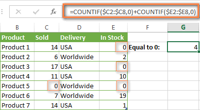
An alternative way is using the INDIRECT function to create an array of ranges. For example, both of the below formulas produce the same result you see in the screenshot:
=SUM(COUNTIF(INDIRECT({"B2:B8","D2:C8"}),"=0"))
=COUNTIF($B2:$B8,0) + COUNTIF($C2:$C8,0)
2. Ampersand and quotes in COUNTIF formulas
Question: When do I need to use an ampersand in a COUNTIF formula?
Answer: It is probably the trickiest part of the COUNTIF function, which I personally find very confusing. Though if you give it some thought, you'll see the reasoning behind it - an ampersand and quotes are needed to construct a text string for the argument. So, you can adhere to these rules:
If you use a number or a cell reference in the exact match criteria, you need neither ampersand nor quotes. For example:
=COUNTIF(A1:A10,10)
or
=COUNTIF(A1:A10,C1)
If your criteria includes text, wildcard character or logical operator with a number, enclose it in quotes. For example:
=COUNTIF(A2:A10,"lemons")
or
=COUNTIF(A2:A10,"*") or =COUNTIF(A2:A10,">5")
In case your criteria is an expression with a cell reference or another Excel function, you have to use the quotes ("") to start a text string and ampersand (&) to concatenate and finish the string off. For example:
=COUNTIF(A2:A10,">"&D2)
or
=COUNTIF(A2:A10,"<="&TODAY())
If you are in doubt whether an ampersand is needed or not, try out both ways. In most cases an ampersand works just fine, e.g. both of the below formulas work equally well.
=COUNTIF(C2:C8,"<=5")
and
=COUNTIF(C2:C8,"<="&5)
3. COUNTIF for formatted (color coded) cells
Question: How do I count cells by fill or font color rather than by values?
Answer: Regrettably, the syntax of the Excel COUNTIF function does not allow using formats as the condition. The only possible way to count or sum cells based on their color is using a macro, or more precisely an Excel User-Defined function. You can find the code working for cells colored manually as well as for conditionally formatted cells in this article - How to count and sum Excel cells by fill and font color.
4. #NAME? error in the COUNTIF formula
Issue: My COUNTIF formula throws a #NAME? error. How can I get it fixed?
Answer: Most likely, you have supplied an incorrect range to the formula. Please check out point 1 above.
5. Excel COUNTIF formula not working
Issue: My COUNTIF formula is not working! What have I done wrong?
Answer: If you have written a formula which is seemingly correct but it does not work or produces a wrong result, start by checking the most obvious things such as a range, conditions, cell references, use of ampersand and quotes.
Be very careful with using spaces in a COUNTIF formula. When creating one of the formulas for this article I was on the verge of pulling my hair out because the correct formula (I knew with certainty it was right!) wouldn't work. As it turned out, the problem was in a measly space somewhere in between, argh... For instance, look at this formula:
=COUNTIF(B2:B13," Lemonade").
At first sight, there is nothing wrong about it, except for an extra space after the opening quotation mark. Microsoft Excel will swallow the formula just fine without an error message, warning or any other indication, assuming you really want to count cells containing the word 'Lemonade' and a leading space.
If you use the COUNTIF function with multiple criteria, split the formula into several pieces and verify each function individually.
And this is all for today. In the next article, we will explore several ways to count cells in Excel with multiple conditions. Hope to see you next week and thanks for reading!
 by
by
1038 comments
Please help me. I'm stuck on the following excel formula:
=IF($H$26="Acting","","",IF($H$26="Temporary","","",IF($H$26="PERMANENT"(VLOOKUP($D$20,'Job Title'!$A$2:$C$28,3,FALSE),""))
“Acting”, “Temporary”, or “Permanent” are text
If H26 is “Acting” or “Temporary” return should be blank
If H26 is “Permanent” it should perform a VLookUP at different D20 and compare it to spreadsheet named Job Title.
Getting error: "The formula you typed contains an error"
Hello,
I have a simple two column worksheet. Column one consists of names, and column two of dates those names were given a task. I need a total that calculates how many times each name was given a task on today's date.
So each day, as the tasks are assigned and entered the total should reflect how many were given to each name that day.
I am trying to use a countifs formula. I have B:B as the Criteria_range1, and =COUNTIF(B:B,TODAY()) as Criteria1, but this doesn't work.
Can somebody tell me what I need to enter to make this calculation work? Any help would be greatly appreciated.
Hi Douglas,
The formula is correct and it worked perfectly on my test sheet. I can think of only reason for it not working - dates formatted as text. Is it the case?
I currently have column B formatted as Date, and chose the 03/14/01 format. :(
Thanks for the help Svetlana. I'm sure it is something minor I am overlooking, but I can't figure it out. I have tried formatting column B as text, date and custom but still cannot get it to work.
Douglas,
Minor things often cause big problems :) If you can send your sample workbook with the formula to our support team (support@ablebits.com) we will try to figure it out.
Svetlana, thanks, that did the trick!!!! You're amazing, and this site is wonderful! Thanks again!!
Nice Article!
I am trying to count occurrences above a certain number; however, those values I want to count are not in a straight row or column. I have each company, then label, then each month in the columns. For each company in the column, I have 4 sets of information. I want to count 1 set for each company. How do I do that?
Sample:
Company A $ of x $50
$ of y $12
# of employees 49
Company B $ of x $150
$ of y $75
# of employees 289
For each company, I want a count of any time the number of employees in that column is greater than 250.
Hello,
I am trying write a function to count the number of unique values in one column that fall in a category in another column.
Here is a simplified example of my data:
Order Qty Group
1 1 1
2 2 1
3 1 1
4 4 1
5 5 2
6 8 2
7 2 2
8 4 2
9 6 2
I want to know how many different/unique order quantities there are within group 1, group 2, etc but without designating the cell range, just the particular value (1 or 2 in this case).
Thanks so much!
________________
|__a_|____b_____|
|poo |480 menit |
|ssp |360 menit |
|LLLL|300 menit |
|LLLL|300 menit |
|____|__________|
so the the result would be like this :
________________
|__a_|____b_____|
|poo |480 menit |
|ssp |360 menit |
|LLLL|600 menit |
|____|__________|
how to do opperation like that ? thanks before
Hi Svetlana,
I have a problem I think can be solved using this method but I cant seem to get the syntax right
I have a list of words in 1 column that have duplicates and a date range in another column
What I need to do is count non duplicates when the date is less then 7 days ago.
the table would look something like this
Apple 26/6/2015
Apple 24/6/2015
Pear 20/6/2015
Pear 15/6/2015
Pear 22/6/2015
Orange27/6/2015
Hi Svetlana,
I am using excel 2003 :(
I am trying to count how many cells in column D contain a specific text, IF the dates in column F are greater than 6 months ago from today.
I have tried this:
=SUMPRODUCT((D4:D16390=D4)*(F4:F16390="<="&TODAY()-180))
But cant seem to get it to work, just shows 0.
Many thanks!
Hi Gary,
Try the following array formula:
=SUM((D4:D16390=D4)*(F4:F16390<=TODAY()-180))
Remember to press Ctrl+Shift+Enter to complete it.
Hi Svetlana,
Perfect! Thank you very much for that!
Hi,
I need to count the amount of profit-making enterprises:
Проект* Выручка Себестоимость
SAMA-001_ALFA 100 90
SAMA-003_BETA 120 200
...
THANK YOU
Count #projects if = Выручка>Сеьестоимость
Hi,
Supposing that "Выручка" is column B and "Себестоимость" is column C, you can use the following array formula:
=SUM(--(B2:B10>C2:C10))
Remember to press Ctrl + Shift + Enter to enter the array formula correctly.
Can you please give me solution for my earlier email?
Please help me to solve my assignment I dont know how...
Count if
A B C
1. 10 20 15
2. 5 25 4
3. 3 6 2
Count if
1) 5-2
2) 1-5
3) 15-25
Hello Nikki,
Here you go:
1) 5-2 =COUNTIFS($A$1:$C$3, "<="&5, $A$1:$C$3, ">="&2)
1) 1-5 =COUNTIFS($A$1:$C$3, "<="&5, $A$1:$C$3, ">="&1)
1) 15-25 =COUNTIFS($A$1:$C$3, "<="&25, $A$1:$C$3, ">="&15)
Hi Svetlana,
I have some data like this in a column. If am giving formula (=COUNTIF(A1:A2000, A1)) to count the number of repetition of each number its not getting counted properly. Its taking into con sideration only few entries. May be coz character are more than 19. Is there any way to count the repetitions if the number of character in a cell is more than 19.
89XXXXXXXXXXXXXXX44
89XXXXXXXXXXXXXXX36
89XXXXXXXXXXXXXXX28
89XXXXXXXXXXXXXXX10
89XXXXXXXXXXXXXXX02
Hi Svetlana,
Looking for an idea for a function. I'm pulling data from one spreadsheet with account numbers assigned to different agents, and trying to compare it to the number of entries made in our sales database for these accounts. The problem is, the database entries contain the account numbers, but also contain other text/numbers as well. Any suggestions? Thank you!
After tinkering around with it, I think the main point of my problem is getting the *value* function to work with a cell reference as the value, rather than a constant.
Hi,
Can you help me out in finding the hours in an column G which is >4 <6 and =6.
time is in 4:00:00 formate and also i need to find no 4 to 6 in same column
Thanks
Shwetha
Hi Shwetha,
You can use the TIME function in your criteria, like this:
Times greater than 4: =COUNTIF(G2:G100, ">"&TIME(4,0,0))
And use analogous formulas for other calculations.
Hi,
I know how to do this using PIVOT, but I have a non power user that will use a template sheet in excel and I'm trying to help him to get a count duplicates cases based on a condition.
Case Cause Dealer
447839 L CA
447839 P CA
447839 S CA
448387 L CA
448387 P CA
447646 L PH
447646 P PH
447647 L PH
447647 P PH
447648 L PH
447648 P PH
In above example CA have 2 cases and PH have 3 cases. Using PIVOT is easy to get the result rather then calculating through transactional data but the user isn't PIVOT oriented and I tried hard to trained.
How I can achieve above summary results using a function/complex formula.
Anticipate thanks,
Jose
Hello,
I have the following data:
Column A Column B Column C
Estimate Percentage Percentage Expected
(days) Complete Remaining Result
0 0 Not Required
5 25 3.25
1 75 .25
Not Required 0 Not Required
So, those fields that are not a number and are equal to zero should not be calculated, but for the formula used to calculate "Percentage Remaining", it is: Column A * (Column B /100)
So, my question is: How do I exclude the calculations that are zeros and are not numbers in Column A and Column B?
Hi, I have a spread sheet where I have a resident name in column A and a hall number in column B. There are multiple residents on the same hall, and sometimes the resident is listed more than once. I want to count the number of times a hall is listed, but no duplicates(i.e Joe 100
Bill 200
Joe 100
Chris 300
Maple 100. So I would want to find out how many times 100 is involved without the duplicate so the count should be 2. Can you help me? thanks,Joe
Hi - I have a baseball schedule and trying to see how many times each team has a early and late game. I have used the countifs but can't get it to work.
Away Team # Vs Home Team # Time and Diamond
1 vs 2 715 P
3 vs 4 845 P
5 vs 6 715 D1
7 vs 8 845 D2
11 vs 12 715 D1
9 vs 10 845 D2
12 vs 1 715 P
10 vs 3 845 P
8 vs 5 715 D1
6 vs 7 845 D2
4 vs 9 715 D1
2 vs 11 845 D2
Thank you, Kendra
Hi Kendra,
And how do you determine whether it's an early and late game?
Hi Miss Svetlana how i could count the total sum of all tools without using pivot example.
Colum A. Colum B.
Description: Total Amount:
Tools & Equipment A 3,000.00
Tools & Equipment B 4,000.00
Tools & Equipment B 1,000,00
Tools & Equipment C 2,500,00
Tools & Equipment D 500,00
Tools & Equipment C 1,500.00
Tools & Equipment E 800.00
Tools & Equipment A 3,800.00
Tools & Equipment E 540.00
Tools & Equipment E 900.00
Tools & Equipment E 100.00
Tools & Equipment E 100.00
Tools & Equipment E 300.00
Tools & Equipment B 6,000.00
Can u help me pls.......
i need to total by each tools without using pivot
Svetlana,
I'm trying to make a formula that does not count any cell that is Blank or 0. What am I missing here? "=-COUNTIF(B5:F5,B6:F6,"<=0"),(B5*B6+C5*C6+D5*D6+E5*E6*F5*F6)/G5" The B5..F6 cells could be blank or 0, but I just want a simple formula that does provides the weighted average.
Thank You!
Johan Bolle
I have summation formulas in column Z and 2 cells with a value > 0
When I use the COUNTIF(Z5:Z108,">0" ) it correctly answers 2
How can I combine that with the question "How many are SHOWN that have a value > 0 somewhat like =Subtotal(109,Z5:Z108)
Unsuccessfully tried
SUBTOTAL(109,COUNTIF(Z5:Z108,">0")) and
COUNTIF(SUBTOTAL(109,Z5:Z108),">0")
Hi Svetlana,
I am using COUNTIF to give me a count of results that are in a range. I want to know how many fall between 8,000 to 9,000, 9,000 to 10,000, and so on. My range of data to look at is A1-A164 but within that range are many subcategories with totals for that category. My COUNTIF counts the total in the results but I don't want the totals counted. Other than making 50 separate ranges is there any other way you can think of to exclude the total cells from being included in the count?
Thank you for any help you can offer.
Hi Debbie,
I am afraid I cannot figure out any way other than you suggested :(
Debbie,
I realize it has been some time since if you inquired; my apologies. If I'm understanding your dilemma properly, is it not possible to use COUNTIFS and ignore rows where the total values have the keyword "Total" in an adjacent column?
I am trying to keep track of attendance of employees for the current month. I have a formula that will calculate the last 30 days for the attendance code, but instead of last 30 days I would like for current month only:
=COUNTIFS(Attendance!$B:$B,$B5,Attendance!$E:$E,"CIO - CI OUT",Attendance!$C:$C,">"&(TODAY()-30))
I have 2 separate sheets - Attendance sheet which is the sheet I log attendance to, and the other sheet where I am placing my formulas on. Here is a breakdown of everything from that formula above
Counts for that employee if it meets all of the following criteria:
**Attendance!$B:$B,$B5 >> Employee Name (want to count specific employee)
**Attendance!$E:$E,"CIO - CI OUT" >> Attendance code (want to count specific attendance code)
**Attendance!$C:$C,">"&(TODAY()-30) >> THIS IS WHAT I NEED TO CHANGE. I need to change instead of being last 30 days, to be for the CURRENT month only.
So today being in May, I want it to count how many times "John Doe" has had the Attendance code of "CIO - CI OUT" for THIS MONTH. It should reset next month to only include June automatically.
Hi Svetlana,
Can you help please?
I am currently using the CountA function to count the cells in a column.
Some cells have ? or * in them.
I have the formula to not count these cells?
How do I achieve this?
Thanks much.
Hi!
You can count the cells with ? and * and then subtract them from the total count, like this:
=COUNTA(A1:A100)-COUNTIF(A1:A100,"~*")-COUNTIF(A1:A100,"~?")
Hi Svetlana,
I have an excel table to keep a running balance of the decreasing loan amount, as payments are made (see excerpt from table below).
Currently, the formula in column D is =SUM(D2,C3) & the formula in column E is =E2-D3
The problem with this is that is when I continue the formula's all the way down to #21 on the list; the $150 in D continues all the was down the list, & the $4,350 in E does the same. It stays that way until I add a new payment to column C; and then the new total continues down the list.
I don't want anything showing in Columns D & E until another payment is made. I want the formula's in there; so the balance automatically adjusts when I enter a payment, but I don't want any value showing if no payment has been made.
I thought I could accomplish this by using a COUNTIF formula.
Something like: If C is greater than zero, then =SUM(D3,C4)& =E3-D4.
I'm not sure how to set the up.
Can you help me with that? Any help would be very much appreciated.
C D E
$ AMOUNT of PMT BALANCE PD TO DATE BALANCE OWING
$0.00 $0.00 $4,500.00
$150.00 $150.00 $4,350.00
Dear Sir/madam,
Please help.
I have a range of codes with some are duplicate in one column. I would like to count the code but for those are duplicate to be counted only one time.
Veasna
i want to know how calculate spreadsheets
my no is this 109|110
109|110
109|110
how many times 109 in this range
I have a spreadsheets that tracks the schedule of my sales rep's from week to week. I have a column set up to count how many total appointments they have per day. In this column I use the formula =COUNTIF(tblMonday[@[9:00 AM]:[5:00 PM]],"*") so it reads all addresses as a count. I have another column set up to count only the warranty appointments for that day. In that column, I am using the formula =COUNTIF(tblMonday[@[9:00 AM]:[5:00 PM]],"(W)*") to recognize that when I type (W) in front of the address, it is a warranty call and will go just to that column. I would like to add a third column that counts only the addresses that have no (W) in front. Please... send help. :-)
I have a table with numbers in Columns F, G, H, I, and J. There is an identifier in Column B.
I need the average of all numbers in Columns F, G, H, I, and J where the identifier in Column B = A14 (i.e. the value in A14).
I tried the following:
=AVERAGEIFS('Hours-Backup'!F3:J1048576,'Hours-Backup'!B:B,'Group Dashboard'!A14)
This results in a #VALUE! error.
I can't figure out what the problem is. Any help would be appreciated.
Ultimately, I want to make it so that the function ignores all cells that are non-numeric or blank. In other words, I don't want it to assume that blank cells are 0 for averaging purposes.
Thanks!
Hi,
I was wondering if it is possible to count partial matches in the following example:
Orange juice
Apple juice
Juice
Coca Cola
So would want the count if formula return 3. I believe if I use *juice it will count only the first two, as "Juice" doesn't have anything in front of it.
Thanks!
Hi Lidiya,
You can use *Juice* and it will count all 3. The asterisk tells the formula to count all instances regardless of the presence or absence of any other characters in front of / after the word.
Hello Svetlana,
I need help with the following problem. I have a column with 4 different values:
Column A
39
19
20
0
20
19
19
19
0
39
19
0
39
19
39
0
0
0
19
39
20
0
20
I need a formula that will count the number of appearances of the number 0 since the last time the number 39 has appeared. Numbers 19 and 20 are not important, but they have to be there. Basically it counts the number of times the lowest value in the column has appeared since the last appearance of the greatest value in the column. The formula will be put in column B and will have to show the following results:
Column B
0
0
0
1
1
1
1
1
2
0
0
1
0
0
0
1
2
3
3
0
0
1
1
Is it possible?
Thanks in advance!
Hi Svetlana Cheusheva
hope your doing well.. please help me out .. i have attached my worksheet with this mail.
i want total value of cells A , B , & C to be calculated in Cell "D" automatically .
please show me step by step..
TERMINAL
PRICE
A
1000
B
2000
TICKET
PRICE
YES
0
NO
150
STAGGING
PRICE
STAGE-1
510
STAGE-2
510
PARKING
0
your support will be highly appreciated
Hi Svetlana,
I am trying to figure out how to formulate a countif function where I am trying to measure exposure on certain loans on any given date. I have a bunch of loans, the amount pertaining to that loan and the respective maturity/expiry date. Essentially, I am trying to measure peak exposure from today lookng forward over the next 5 years so that I can create a graph in excel illustrating exposure over time. I would like the graph to show me how much exposure I have to those loans in year 3 in quarter 4 and how many have been repaid.
Do you have any idea how I might do so?
Many thanks in advance,
Ben
Hey, great post, and thanks for the pointers! I have a basic timesheet for work and would like to count the days spent on each project. Are you able to tell me how I can redirect the condition to another cell? So that:
=COUNTIF(timesheet!$C$4:$G$500,"project A")
would become:
=COUNTIF(timesheet!$C$4:$G$500,"cell reference that redirects to the beginning of the row, which is where the project is named")
This way, I will be able to remove the need to enter the project name twice and the risk of an error due to billing days for project A against project B.
Thanks!
Hi,
Is there any way we can figure out a formulae for this tracker. Basically tracker should automatically calculate the blood samples drawn 12 months from the day they signed the consent form.
Eg- if patient signed consent in 27/07/2013 and the bloods are drawn until end of JULY 2014, the tracker should calculate signed consent + 365 days.
Thanks a lot in advance.
Hi Sat,
I think it is possible. For me to be able to suggest a formula, please explain the structure of your data, i.e. what columns contain signed consent dates and blood drown dates and probably patients' names. Also, what exactly you want to get as a result - the expiry date for each blood sample or something different?
Hi Svetlana,
Thank you for publishing this page and always being active to respond.
I am stuck with a Problem :
Query : Count of projects between 01/01/2015 and 01/31/2015 whose status is ABC OR XYZ.
From your forum I could do it for Count of project Less than 01/31/2015 but that will include all 2014 and 2013 projects also.
I used the following formula for this :
=COUNTIFS(Details!D17:D33,"<01/31/2015", Details!E17:E33, "ABC")+COUNTIFS(Details!D17:D33,"<12/31/2014", Details!E17:E33, "XYZ")
Could you please help out with date range for this.
Hi Svetlana,
Thank you for this very helpful topic!
I have this question: Is it possible with a formula to count all the rows from A to D in which the sum of the cells is greater than 0 and between 4.
For example in this case, the result will be 2 :
A B C D E
1 0 1 5 0 4
2 0 3 12 0 0
3 0 1 2 0 1
4 7 2 5 0 2
5 0 0 0 1 4
Thank you very much,
Elena
Hi Elena,
Sorry, I am a bit confused. Do you mean the sum of values in columns A through D in each row, e.g. A1:D1, A2:D2, etc.? If so, it is always greater than 0 and even greater than 4 in your example. Please clarify.
I want to know whether its possible to calculate and if yes what are the tags to find out whether the values have crossed the certain threshold and if it does can the names of whoever has crossed can be displayed
Hi,
I need to count the number of hours for midnight charge given the criteria to be 11pm to 6am.
E.g.(1) Cell A1 9pm and cell B1 9am. the result for midnight hours should be 7hrs
E.g.(2) Cell B1 12am and cell B2 10am. the result for midnight hours should be 6hrs.
How should i input the formula?
thank you very much.
how to count a data by date but including text contain like
A columns
1-Mar-15
6-Mar-15
11-Mar-15
16-Mar-15
21-Mar-15
26-Mar-15
31-Mar-15
a
a
how do i take all the count
Hi Shoaib,
Not sure if I understand the task correctly. Anyway, if you want to count all cells with any data in column A, you can use the following formula:
=COUNTIF(A2:A100,"<>"&"")
Please see the example in the "Count if blank or not blank" for full details.
Hi
I want to know whether it is possible to get the count of cells that are not empty.
Hi Athi,
Of course, this is possible. Please check out the following examples:
Count blanks and non-blanks
I am trying to count how may times Toronto plays a game in the U10 age group.
Column A = Age group
Column B = Home Team
Column C = vs
Column D = Away Team
Age Group Team 1 Team 2
U8 Moncton vs Halifax
U9 Toronto vs Moncton
U10 Moncton vs Halifax
U12 Halifax vs Vancouver
U8 Toronto vs Vancouver
U9 Halifax vs Toronto
U10 Toronto vs Vancouver
U12 Vancouver vs Moncton
U8 Vancouver vs Halifax
U9 Toronto vs Moncton
U10 Moncton vs Vancouver
U12 Vancouver vs Moncton
U8 Vancouver vs Toronto
U9 Moncton vs Vancouver
U10 Toronto vs Moncton
U12 Halifax vs Fredericton
if any cell in column b equals a certain text then count cells in column c
post jan feb mar apr may
admin 10 20
admin 25 2
asst manager 10 17
asst manager 2 28
bartender 21
bartender 30
captain 15 15
captain 13 17
hostess 10 15
hostess 25 5
manager 16 14
manager 30
manager 25 3
manager 20 2
supervisor 20 10
supervisor 15 15
waiter 25
waiter 30
waiter 20
waiter 18
waiter 10
waiter 14 13
waiter 20
waiter 25
waiter 28
waiter 30
waiter 15
8 8 11 10 4
admin 1
asst manager 1
bartender 1
captain 0
hostess 1
manager 1
supervisor 1
waiter 2
Total 8 0 0 0 0
Hi,
I want to format Column A of a sheet. Column A has names and in columns B:M are the 12 numbers (1-75) associated to each name. In Q1:Z30 I have up to (depending on the day) 300 random numbers 1-75. I need the name in Column A to turn Pink when 9 of the numbers match the numbers entered in Q1:Z30. Since there are up to 300 numbers entered in Q1:Z30, some numbers are entered more than once. Here is the Conditional Formatting formula that I am using that isn't working:
=SUM(COUNTIF($B1:$M1,$Q$1:$Z$30))>=9
The formula is counting each instance that it matches and adding those up, and when those 12 numbers have been matched 9 times it highlights the name in Column A. I need the formula to highlight when 9 of the numbers in B:M have been matched period, not how many times they have been matched.
Thank you so much for your time!
Hello,
I need help with function Countif, so:
I want to count two cells for example: if cell A1=1 or cell A2=1 so count as 1, if one of these cells equal 1, count as 1, if both cells equal 1, count 1 as well. How is it possible to do with function Countif or with other function?
Thank you in advance
I have two columns. I would like to count the the no. of values in the right column greater greater than the corresponding values in left column. How to accomplish this?
Hi Svetlana - Hope you are fine, required small help from you, is there any formula to capture code from statment by using if formula. I have 34 Codes, need to capture below code if they come in different entries, Example for entry : XXXXXXXXXXXXXXXXXXXXXXXXXXXXXXX & /AC04/ XXXXXXXXXXXXXXXXXXX, in this case AC04 is code. want to capture below code by using if formula, they can start AC or AM or BE or AG or BT or MS or PY or RS.
1 AC01
2 AC02
3 AC03
4 AC04
5 AC05
6 AC06
7 AM01
8 AM02
9 AM03
10 AM04
11 AM05
12 AM06
13 AM07
14 AM08
15 BE01
16 BE02
17 BE03
18 BE04
19 BE05
20 AG01
21 AG02
22 DT01
23 MS01
24 PY01
25 RF01
26 RC01
27 RC02
28 RC03
29 RC04
30 RR01
31 RR02
32 RR03
33 TM01
34 X1!c2!n
Please can you advise a formula for this.
Thanks & Regards
Ashish Baddar
Hi there,
Good day to you, i have a XLS with 2 Tab Aging and score card. I have different value for column "W" in aging tab and i would like calculate the below.
1. to calculate the total for all the different texts which are not "abc" and with a specific aging day.
** Please Help**
2. to calculate the total "abc" and with a specific aging day, which i mange to do it.
=COUNTIFS(Aging!$W:$W,"abc",Aging!$B:$B,ScoreCard!J18,Aging!$N:$N,"<15")
Hello i am having a Count if issue
the formula i am using is:
=OFFSET('Raw Data'!$K$5,1,0,COUNTIF('Raw Data'!$K:$K,">0"))
i am using this in name manager to automatically update a control chart as i dump data in my "Raw Data" tab.
the chart is a representation of a shipments date (x axis) and the analysis of the shipment on that date.
the issue that i am having is that the formula is not counting the entire column. Furthermore my chart is still picking up the zeros
there is a large amount of entries in the column (J5-J65 the formula above stops at J26. i can not figure out why.
Im sorry
in the range above i mean K5-K65 and stops a K26
You're really great!!