Microsoft Excel provides several functions purposed for counting different kinds of cells, such as blanks or non-blanks, with number, date or text values, containing specific words or character, etc.
In this article, we will focus on the Excel COUNTIF function that is purposed for counting cells with the condition you specify. First, we will briefly cover the syntax and general usage, and then I provide a number of examples and warn about possible quirks when using this function with multiple criteria and specific types of cells.
In essence, COUNTIF formulas are identical in all Excel versions, so you can use the examples from this tutorial in Excel 365, 2021, 2019, 2016, 2013, 2010 and 2007.
COUNTIF function in Excel - syntax and usage
Excel COUNTIF function is used for counting cells within a specified range that meet a certain criterion, or condition.
For example, you can write a COUNTIF formula to find out how many cells in your worksheet contain a number greater than or less than the number you specify. Another typical use of COUNTIF in Excel is for counting cells with a specific word or starting with a particular letter(s).
The syntax of the COUNTIF function is very simple:
As you see, there are only 2 arguments, both of which are required:
- range - defines one or several cells to count. You put the range in a formula like you usually do in Excel, e.g. A1:A20.
- criteria - defines the condition that tells the function which cells to count. It can be a number, text string, cell reference or expression. For instance, you can use the criteria like these: "10", A2, ">=10", "some text".
And here is the simplest example of Excel COUNTIF function. What you see in the image below is the list of the best tennis players for the last 14 years. The formula =COUNTIF(C2:C15,"Roger Federer") counts how many times Roger Federer's name is on the list:
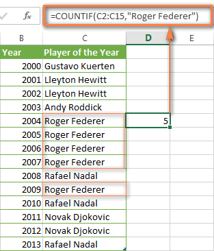
Note. A criterion is case insensitive, meaning that if you type "roger federer" as the criteria in the above formula, this will produce the same result.
Excel COUNTIF function examples
As you have just seen, the syntax of the COUNTIF function is very simple. However, it allows for many possible variations of the criteria, including wildcard characters, the values of other cells, and even other Excel functions. This diversity makes the COUNTIF function really powerful and fit for many tasks, as you will see in the examples that follow.
COUNTIF formula for text and numbers (exact match)
In fact, we discussed the COUNTIF function that counts text values matching a specified criterion exactly a moment ago. Let me remind you that formula for cells containing an exact string of text: =COUNTIF(C2:C15,"Roger Federer"). So, you enter:
- A range as the first parameter;
- A comma as the delimiter;
- A word or several words enclosed in quotes as the criteria.
Instead of typing text, you can use a reference to any cell containing that word or words and get absolutely the same results, e.g. =COUNTIF(C1:C9,C7).
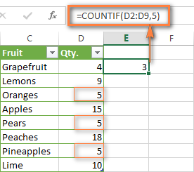
Similarly, COUNTIF formulas work for numbers. As shown in the screenshot below, the below formula perfectly counts cells with quantity 5 in Column D:
=COUNTIF(D2:D9, 5)
In this article, you will find a few more formulas to count cells that contain any text, specific characters or only filtered cells.
COUNTIF formulas with wildcard characters (partial match)
In case your Excel data include several variations of the keyword(s) you want to count, then you can use a wildcard character to count all the cells containing a certain word, phrase or letters as part of the cell's contents.
Suppose, you have a list of tasks assigned to different persons, and you want to know the number of tasks assigned to Danny Brown. Because Danny's name is written in several different ways, we enter "*Brown*" as the search criteria =COUNTIF(D2:D10, "*Brown*").
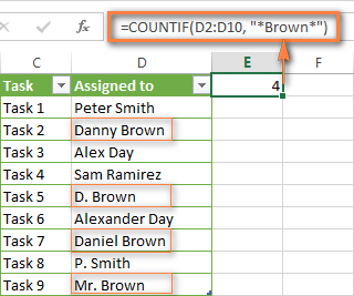
An asterisk (*) is used to find cells with any sequence of leading and trailing characters, as illustrated in the above example. If you need to match any single character, enter a question mark (?) instead, as demonstrated below.
Tip. It is also possible to use wildcards with cell references with the help of the concatenation operator (&). For example, instead of supplying "*Brown*" directly in the formula, you can type it in some cell, say F1, and use the following formula to count cells containing "Brown": =COUNTIF(D2:D10, "*"&F1&"*")
Count cells beginning or ending with certain characters
You can use either wildcard character, asterisk (*) or question mark (?), with the criterion depending on which exactly result you want to achieve.
If you want to know the number of cells that start or end with certain text no matter how many other characters a cell contains, use these formulas:
=COUNTIF(C2:C10,"Mr*") - count cells that begin with "Mr".
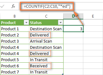
=COUNTIF(C2:C10,"*ed") - count cells that end with the letters "ed".
The image below demonstrates the second formula in action:
If you are looking for a count of cells that start or end with certain letters and contain the exact number of characters, you use the Excel COUNTIF function with the question mark character (?) in the criteria:
=COUNTIF(D2:D9,"??own") - counts the number of cells ending with the letters "own" and having exactly 5 characters in cells D2 through D9, including spaces.
=COUNTIF(D2:D9,"Mr??????") - counts the number of cells starting with the letters "Mr" and having exactly 8 characters in cells D2 through D9, including spaces.
Tip. To find the number of cells containing an actual question mark or asterisk, type a tilde (~) before the ? or * character in the formula. For example, =COUNTIF(D2:D9,"*~?*") will count all cells containing the question mark in the range D2:D9.
Excel COUNTIF for blank and non-blank cells
These formula examples demonstrate how you can use the COUNTIF function in Excel to count the number of empty or non-empty cells in a specified range.
COUNTIF not blank
In some Excel COUNTIF tutorials and other online resources, you may come across formulas for counting non-blank cells in Excel similar to this one:
=COUNTIF(A1:A10,"*")
But the fact is, the above formula counts only cells containing any text values including empty strings, meaning that cells with dates and numbers will be treated as blank cells and not included in the count!
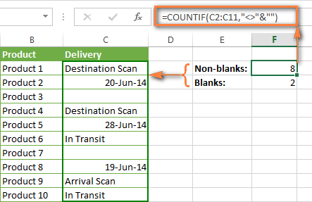
If you need a universal COUNTIF formula for counting all non-blank cells in a specified range, here you go:
Or
This formula works correctly with all value types - text, dates and numbers - as you can see in the screenshot below.
COUNTIF blank
If you want the opposite, i.e. count blank cells in a certain range, you should adhere to the same approach - use a formula with a wildcard character for text values and with the "" criteria to count all empty cells.
Formula to count cells not containing any text:
Since an asterisk (*) matches any sequence of text characters, the formula counts cells not equal to *, i.e. not containing any text in the specified range.
Universal COUNTIF formula for blanks (all value types):
The above formula correctly handles numbers, dates and text values. For example, here's how you can get the number of empty cells in the range C2:C11:
=COUNTIF(C2:C11,"")
Please be aware that Microsoft Excel has another function for counting blank cells, COUNTBLANK. For instance, the following formulas will produce exactly the same results as the COUNTIF formulas you see in the screenshot above:
Count blanks:
=COUNTBLANK(C2:C11)
Count non-blanks:
=ROWS(C2:C11)*COLUMNS(C2:C11)-COUNTBLANK(C2:C11)
Also, please keep in mind that both COUNTIF and COUNTBLANK count cells with empty strings that only look blank. If you do not want to treat such cells as blanks, use "=" for criteria. For example:
=COUNTIF(C2:C11,"=")
For more information about counting blanks and not blanks in Excel, please see:
COUNTIF greater than, less than or equal to
To count cells with values greater than, less than or equal to the number you specify, you simply add a corresponding operator to the criteria, as shown in the table below.
Please pay attention that in COUNTIF formulas, an operator with a number are always enclosed in quotes.
| Criteria | Formula Example | Description |
|---|---|---|
| Count if greater than | =COUNTIF(A2:A10,">5") | Count cells where value is greater than 5. |
| Count if less than | =COUNTIF(A2:A10,"<5") | Count cells with values less than 5. |
| Count if equal to | =COUNTIF(A2:A10,"=5") | Count cells where value is equal to 5. |
| Count if not equal to | =COUNTIF(A2:A10,"<>5") | Count cells where value is not equal to 5. |
| Count if greater than or equal to | =COUNTIF(C2:C8,">=5") | Count cells where value is greater than or equal to 5. |
| Count if less than or equal to | =COUNTIF(C2:C8,"<=5") | Count cells where value is less than or equal to 5. |
You can also use all of the above formulas to count cells based on another cell value, you will just need to replace the number in the criteria with a cell reference.
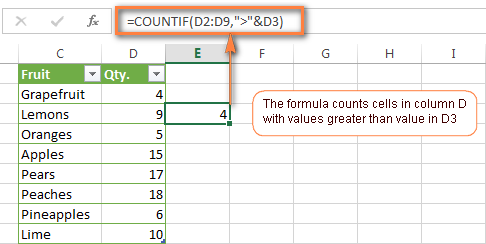
Note. In case of a cell reference, you have to enclose the operator in quotes and add an ampersand (&) before the cell reference. For example, to count cells in the range D2:D9 with values greater than a value in cell D3, you use this formula =COUNTIF(D2:D9,">"&D3):
If you want to count cells that contain an actual operator as part of the cell's contents, i.e. the characters ">", "<" or "=", then use a wildcard character with the operator in the criteria. Such criteria will be treated as a text string rather than a numeric expression. For example, the formula =COUNTIF(D2:D9,"*>5*") will count all cells in the range D2:D9 with contents like this "Delivery >5 days" or ">5 available".
Using Excel COUNTIF function with dates
If you want to count cells with dates that are greater than, less than or equal to the date you specify or date in another cell, you proceed in the already familiar way using formulas similar to the ones we discussed a moment ago. All of the above formulas work for dates as well as for numbers. Let me give you just a few examples:
| Criteria | Formula Example | Description |
|---|---|---|
| Count dates equal to the specified date. | =COUNTIF(B2:B10,"6/1/2014") | Counts the number of cells in the range B2:B10 with the date 1-Jun-2014. |
| Count dates greater than or equal to another date. | =COUNTIF(B2:B10,">=6/1/2014") | Count the number of cells in the range B2:B10 with a date greater than or equal to 6/1/2014. |
| Count dates greater than or equal to a date in another cell, minus x days. | =COUNTIF(B2:B10,">="&B2-"7") | Count the number of cells in the range B2:B10 with a date greater than or equal to the date in B2 minus 7 days. |
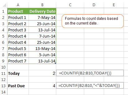
Apart from these common usages, you can utilize the COUNTIF function in conjunction with specific Excel Date and Time functions such as TODAY() to count cells based on the current date.
| Criteria | Formula Example |
|---|---|
| Count dates equal to the current date. | =COUNTIF(A2:A10,TODAY()) |
| Count dates prior to the current date, i.e. less than today. | =COUNTIF(A2:A10,"<"&TODAY()) |
| Count dates after the current date, i.e. greater than today. | =COUNTIF(A2:A10,">"&TODAY()) |
| Count dates that are due in a week. | =COUNTIF(A2:A10,"="&TODAY()+7) |
| Count dates in a specific date range. | =COUNTIF(B2:B10, ">=6/1/2014")-COUNTIF(B2:B10, ">6/7/2014") |
Here is an example of using such formulas on real data (at the moment of writing today was 25-Jun-2014):
Excel COUNTIF with multiple criteria
In fact, Excel COUNTIF function is not exactly designed to count cells with multiple criteria. In most cases, you'd use its plural counterpart, the COUNTIFS function to count cells that match two or more criteria (AND logic). However, some tasks can be solved by combining two or more COUNTIF functions in one formula.
Count values between two numbers
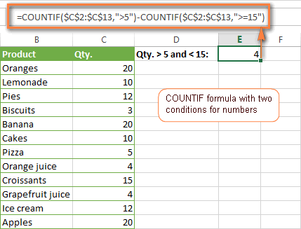
One of the most common applications of Excel COUNTIF function with 2 criteria is counting numbers within a specific range, i.e. less than X but greater than Y. For example, you can use the following formula to count cells in the range B2:B9 where a value is greater than 5 and less than 15.
=COUNTIF(B2:B9,">5")-COUNTIF(B2:B9,">=15")
How this formula works:
Here, we use two separate COUNTIF functions - the first one finds out how many values are greater than 5 and the other one gets a count of values greater than or equal to 15. Then, you subtract the latter from the former and get the desired result.
Count cells with multiple OR criteria
In situations when you want to get several different items in a range, add 2 or more COUNTIF functions together. Supposing, you have a shopping list and you want to find out how many soft drinks are included. To have it done, use a formula similar to this:
=COUNTIF(B2:B13,"Lemonade")+COUNTIF(B2:B13,"*juice")
Please pay attention that we've included the wildcard character (*) in the second criterion, it is used to count all kinds of juice on the list.
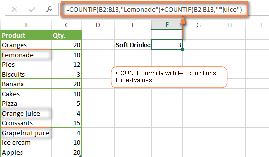
In the same manner, you can write a COUNTIF formula with several conditions. Here is an example of the COUNTIF formula with multiple OR conditions that counts lemonade, juice and ice cream:
=COUNTIF(B2:B13,"Lemonade") + COUNTIF(B2:B13,"*juice") + COUNTIF(B2:B13,"Ice cream")
For other ways to count cells with OR logic, please see this tutorial: Excel COUNTIF and COUNTIFS with OR conditions.
Using COUNTIF function to find duplicates and unique values
Another possible usage of the COUNTIF function in Excel is for finding duplicates in one column, between two columns, or in a row.
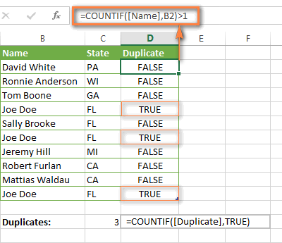
Example 1. Find and count duplicates in 1 column
For example, this simple formula =COUNTIF(B2:B10,B2)>1 will spot all duplicate entries in the range B2:B10 while another function =COUNTIF(B2:B10,TRUE) will tell you how many dupes are there:
Example 2. Count duplicates between two columns
If you have two separate lists, say lists of names in columns B and C, and you want to know how many names appear in both columns, you can use Excel COUNTIF in combination with the SUMPRODUCT function to count duplicates:
=SUMPRODUCT((COUNTIF(B2:B1000,C2:C1000)>0)*(C2:C1000<>""))
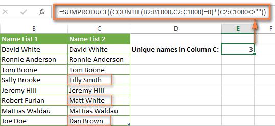
We can even take a step further and count how many unique names there are in Column C, i.e. names that do NOT appear in Column B:
=SUMPRODUCT((COUNTIF(B2:B1000,C2:C1000)=0)*(C2:C1000<>""))
Tip. If you want to highlight duplicate cells or entire rows containing duplicate entries, you can create conditional formatting rules based on the COUNTIF formulas, as demonstrated in this tutorial - Excel conditional formatting formulas to highlight duplicates.
Example 3. Count duplicates and unique values in a row
If you want to count duplicates or unique values in a certain row rather than a column, use one of the below formulas. These formulas might be helpful, say, to analyze the lottery draw history.
Count duplicates in a row:
=SUMPRODUCT((COUNTIF(A2:I2,A2:I2)>1)*(A2:I2<>""))
Count unique values in a row:
=SUMPRODUCT((COUNTIF(A2:I2,A2:I2)=1)*(A2:I2<>""))

Excel COUNTIF - frequently asked questions and issues
I hope these examples have helped you to get a feel for the Excel COUNTIF function. If you've tried any of the above formulas on your data and were not able to get them to work or are having a problem with the formula you created, please look through the following 5 most common issues. There is a good chance that you will find the answer or a helpful tip there.
1. COUNTIF on a non-contiguous range of cells
Question: How can I use COUNTIF in Excel on a non-contiguous range or a selection of cells?
Answer: Excel COUNTIF does not work on non-adjacent ranges, nor does its syntax allow specifying several individual cells as the first parameter. Instead, you can use a combination of several COUNTIF functions:
Wrong: =COUNTIF(A2,B3,C4,">0")
Right: =COUNTIF(A2,">0") + COUNTIF(B3,">0") + COUNTIF(C4,">0")
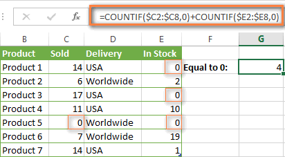
An alternative way is using the INDIRECT function to create an array of ranges. For example, both of the below formulas produce the same result you see in the screenshot:
=SUM(COUNTIF(INDIRECT({"B2:B8","D2:C8"}),"=0"))
=COUNTIF($B2:$B8,0) + COUNTIF($C2:$C8,0)
2. Ampersand and quotes in COUNTIF formulas
Question: When do I need to use an ampersand in a COUNTIF formula?
Answer: It is probably the trickiest part of the COUNTIF function, which I personally find very confusing. Though if you give it some thought, you'll see the reasoning behind it - an ampersand and quotes are needed to construct a text string for the argument. So, you can adhere to these rules:
If you use a number or a cell reference in the exact match criteria, you need neither ampersand nor quotes. For example:
=COUNTIF(A1:A10,10)
or
=COUNTIF(A1:A10,C1)
If your criteria includes text, wildcard character or logical operator with a number, enclose it in quotes. For example:
=COUNTIF(A2:A10,"lemons")
or
=COUNTIF(A2:A10,"*") or =COUNTIF(A2:A10,">5")
In case your criteria is an expression with a cell reference or another Excel function, you have to use the quotes ("") to start a text string and ampersand (&) to concatenate and finish the string off. For example:
=COUNTIF(A2:A10,">"&D2)
or
=COUNTIF(A2:A10,"<="&TODAY())
If you are in doubt whether an ampersand is needed or not, try out both ways. In most cases an ampersand works just fine, e.g. both of the below formulas work equally well.
=COUNTIF(C2:C8,"<=5")
and
=COUNTIF(C2:C8,"<="&5)
3. COUNTIF for formatted (color coded) cells
Question: How do I count cells by fill or font color rather than by values?
Answer: Regrettably, the syntax of the Excel COUNTIF function does not allow using formats as the condition. The only possible way to count or sum cells based on their color is using a macro, or more precisely an Excel User-Defined function. You can find the code working for cells colored manually as well as for conditionally formatted cells in this article - How to count and sum Excel cells by fill and font color.
4. #NAME? error in the COUNTIF formula
Issue: My COUNTIF formula throws a #NAME? error. How can I get it fixed?
Answer: Most likely, you have supplied an incorrect range to the formula. Please check out point 1 above.
5. Excel COUNTIF formula not working
Issue: My COUNTIF formula is not working! What have I done wrong?
Answer: If you have written a formula which is seemingly correct but it does not work or produces a wrong result, start by checking the most obvious things such as a range, conditions, cell references, use of ampersand and quotes.
Be very careful with using spaces in a COUNTIF formula. When creating one of the formulas for this article I was on the verge of pulling my hair out because the correct formula (I knew with certainty it was right!) wouldn't work. As it turned out, the problem was in a measly space somewhere in between, argh... For instance, look at this formula:
=COUNTIF(B2:B13," Lemonade").
At first sight, there is nothing wrong about it, except for an extra space after the opening quotation mark. Microsoft Excel will swallow the formula just fine without an error message, warning or any other indication, assuming you really want to count cells containing the word 'Lemonade' and a leading space.
If you use the COUNTIF function with multiple criteria, split the formula into several pieces and verify each function individually.
And this is all for today. In the next article, we will explore several ways to count cells in Excel with multiple conditions. Hope to see you next week and thanks for reading!
 by
by
1038 comments
Hi there,
For my homework assignment I'm supposed to be using countif for data on earnings for various companies. In one column she wants me to be able to have each value say if it's over $1billion or below, and if it's below, by how much. I am confused on how to do this in one column. She also wants it to display text of my choosing, which I would say "Above" or "below"
Hi i have a spreadsheet Songs and i need to use Simplex criteria to get the names of the row, which formula do i use?
Hello!
Please describe your problem in more detail. Write an example of the source data and the result you want to get. It’ll help me understand it better and find a solution for you. Thank you.
Hi there! I am trying to combine these formulas so that both criteria must be true for it to be counted however as my ranges are different sizes this is problematic with the countif function. Is there a way around this?
These are the two formulas which need to be combined:
=COUNTIF('Volunteer Call Handler Form APRIL'!Q:V,"XXXXXXX - recent")
AND
COUNTIF('Volunteer Call Handler Form APRIL'!G:G,"Inbound")
Hello Tilly!
You can use the COUNTIFS function. But уach additional range must have the same number of rows and columns as the criteria_range1 argument. The ranges do not have to be adjacent to each other. Read about it here.
Hi, I want to count those items which have 3 letters + 4 numbers from below, how to count it please?
ABC2001
ABC2002
ABC2003
ABC2004
ABC2005
ABC2006
ABC2007
ABC2008
ABC20A
ABC20B
ABC20C
ABC2009
ABC2010
ABC2011
Hello,
Please try the following formula:
=SUMPRODUCT(--NOT(ISNUMBER(--LEFT(C1:C14,1))), --NOT(ISNUMBER(--LEFT(C1:C14,2))), --NOT(ISNUMBER(--LEFT(C1:C14,1))), --ISNUMBER(--RIGHT(C1:C14,1)), --ISNUMBER(--RIGHT(C1:C14,2)), --ISNUMBER(--RIGHT(C1:C14,3)), --ISNUMBER(--RIGHT(C1:C14,4)))
I hope it’ll be helpful.
Sorry, not sure what happened to what I typed above. Edited:
Hello, I am trying to count the number of cells within a range of cells that fall between two values. So my values which range between 1000 and 50000 are located in cells I2 through I21. I put a value of 5000 in N4 and 25000 in O4. I want to count how many times the values in cells I2 through I21 fall between 5000 and 25000.
When I use this formula: =COUNTIF(I2:I21,">="&N4)+COUNTIF(I2:I21,"="&N4) I get 27.
When I use =COUNTIF(I2:I21,">="&N4)+COUNTIF(I2:I21,"="&N4) I get 3.
I can count the cells and see that the answer should be 7. 7 out of 20 cells fall between 5000 and 25000.
Thank you.
Hello Adina!
See answer above
Hello, I am trying to count the number of cells within a range of cells that fall between two values. So my values which range between 1000 and 50000 are located in cells I2 through I21. I put a value of 5000 in N4 and 25000 in O4. I want to count how many times the values in cells I2 through I21 fall between 5000 and 25000.
When I use this formula: =COUNTIF(I2:I21,">="&N4)+COUNTIF(I2:I21,"="&N4)-COUNTIF(I2:I21,"<="&O4) I get 3. This is also incorrect because I can count the cells and see that the answer should be 7. 7 out of 20 cells fall between 5000 and 25000.
Thank you.
Hello Adina!
If I understand your task correctly, maybe the following formula should work for you:
=COUNTIF(I2:I21," >= "&N4)-COUNTIF(I2:I21," > "&O4)
or
=SUMPRODUCT(--(I2:I21>=N4),--(I2:I21<=O4))
If there is anything else I can help you with, please let me know.
Hello,
I am trying to count the instances where a particular string of text is found in column A, and the date in column D is within a specific range. Could anyone tell me why this isn't working?
=COUNTIFS(Datasheet!A:A,"*theme*",Datasheet!D:D,">=6/1/2019", Datasheet!D:D,"<=6/30/2019")
Thank you!
Hello Madeline!
Please try the following formula:
=COUNTIFS(A1:A40,"*theme*", D1:D40,">="&DATE(2019,6,1), D1:D40,"<="&DATE(2019,6,30))
Hope you’ll find this information helpful.
Hi i just seek your assistance, i am trying to count the number of request i've send to a specific person in a day and also the number of answer i receive with them i day also. Here's my problem my formula doesn't count right. Here's my formula in Sheet1 (=COUNTIFS(March!O:O,">=" & Summary!B5,March!O:O,"<=" & Summary!B5+1)) details are from Sheet2 with a date and time format for March. Summary!B5 means the day today or next day. Hope you can assist me thanks.
Hi there.
I have data with students performance in a particular classroom.
Data Columns: Names, Age, Gender, class/grade, Attendence, Performance status, performance status update.
Options of performance status / update are: poor, good, excellent.
I want to run some queries on this data in a summary table giving the following information:
1. Count Attendance by: Age, Gender and Class/Grade
2. Count Performance by: Age, Gender, Class/Grade whereby I count Performance Update when both Performance Status and Update have values and count performance status when Update is blank.
Please help. I was thinking of using class/grade as a filter for the summary table such that I can switch between classes easily as well as having overall school summary
This is FABULOUS! Thanks!
I am trying to count the number of shifts a person works between a date range, but the shifts are on a 4 on, 4 off schedule.
In a separate tab, I have the start & end dates of each of the shifts till the end of the year. How do I tell it to count the number of days that someone would work, on this shift, given their start & end date of employment.
The `COUNTIF(range,""&"")` will fail in situation like this: A1 = "abcd", A2 = "1234", A3 = IF(COUNTA(A1)>0, "", A1). The result will be 3 which is wrong because A3 is technically a blank cell.
Hello, I really hope someone can help me,m this has come up a few times at work and we really cannot figure it out!! we want a formula for 2 columns, so.. if column A says 'apple' to count it, but only count it if column B is greater than 60.
I hope someone can help me!!
c column is differnt date and the f column is number..
i want to search how many blanks cell of column c date..
example
c column f column]
07-02-2020 23565
07-02-2020 2454
07-02-2020
08-02-2020
08-02-2020 251454
08-02-2020
07 february 01 cell empty and 08 february 02 cell
I would like to count values based on dates with 2 criteria's.
I need the count of unique tickets worked by agent on single day
(If same ticket is repeated multiple times on single day it should count as one but if same tickets is worked on different date then it should increment by 1.
Please help.
The formula used here is counting unique tickets for whole month
Formula used: 2 attempts made but same result
1st attempt : =SUM(IF((H6=$H$6:$H$27)*($E$6:$E$27<=DATE(2020, 1, 31)), 1/COUNTIFS($H$6:$H$27, H6, $F$6:$F$27, $F$6:$F$27, $E$6:$E$27, "<="&DATE(2020, 1, 31)), ""))
2nd attempt: =SUM(--(FREQUENCY(IF(H6=$H$6:$H$25, COUNTIF($F$6:$F$25, "<"&$F$6:$F$25), ""), (COUNTIF($F$6:$F$25, "0))
(wrong value)
Date TICKETS DISPATCHED ASSIGNEE Total ticket Correct value(to be)
2020-01-24 INC123 Pretty Deena Mathew 2 3
2020-01-24 INC123 Pretty Deena Mathew 2 3
2020-01-25 INC123 Pretty Deena Mathew 2 3
2020-01-24 inc1234 Pretty Deena Mathew 2 3
2020-01-25 ritm012 Rachit Sharma 1 1
Here, first 2 rows value should count 2 as same ticket is worked on single day by one agent,
3rd row should be counting 3 as same ticket is worked on NEXT DAY..
This is very important to resolve.
Please assist
Thanks in advance
What if I'm counting less than / greater than / equal to between times? I have an expected arrival time (column D) and an actual arrival time (column I) listed in HH:MM:SS time and I need to know how many groups arrived before after or exactly when they expected.
Bonus points if I can add another criteria to account for the type of visit ( SGV, Program*, Group)
Hello,
I have a table with a range of cells in one column that I want to count from one cell.
i.e Column P cells 1 through 10, each cell represents a repair number "P1 = Repair 1, P2 = Repair 2 etc etc.
In this range I want all cells to count if the repair numbers are in one other cell ie if cell Q1 has 1, 2, 3, 4, 5, 6 typed in it I would like cell P1, P2, P3, P4, P5, P6 to each show 1. Then if cell Q2 has the same 1 through 6 typed same as Q1 I want cells P1 through P6 to each show 2.
Hope you can help
Gavin.
A1 AHU
A2 AHU
A3 Boiler
A4 Boiler
A5 Boiler
A6 Chiller
A7 Chiller
A8 Chiller
A9 Chiller
A10 Chiller
How to count that How much AHU,Chiller & Boiler in my sheet. I Have 1000 Data in sheet.
Hi there! If you require to know how many of each "AHU", "Boiler" and "Chiller" are in your column, then I hope you find this useful.
In cell A1, let's assume there is a "Product Type" header. In cell B2, create a "AHU" header. In cell C2, create a "Boiler" header. In cell D2, create a "Chiller" header. The headers in cells B2, C2 and D2 will be your target cell references.
Let's assume "AHU" is in cell A2, "AHU" is in cell A3, "Boiler" is in cell A4, etc.
To count the total number of "AHU" in column A, the formula is: =COUNTIF(A:A,$B$1) the result should be 2. To count the total number of "Boiler" in column A, the formula is: =COUNTIF(A:A,$C$1) - the result should be 3. To count the total number of "Chiller" in column A, the formula is: =COUNTIF(A:A,$D$1) - the result should be 5.
I have 4 employees that maintain multiple properties monthly. I need a formula that will calculate how many properties are still needing completed per employee. I have the employees in one column and dates completed in a different column. I need it to count the blanks for each individual employee.
This is wrong:
=COUNTIF(B2:B9,">5")-COUNTIF(B2:B9,">=15")
It should be:
=COUNTIF(B2:B9,">5")-COUNTIF(B2:B9,"<=15")
Please update.
Hi John,
Just test both formulas on any sample data, and you will see which one is correct :)
I would like to know the answer:
How to count the number of leaves in a year using a formula. Like how to capture those dates that I have taken as leave.
Thank you for being very helpful, I am looking for an answer to my question, Is there a formula to this situation?
Name Amt
AA 40
DD 45
AA 48
GG
SS 54
AA 67
GG 85
AA
AA 12
KK
AA 6
LL 15
AA
QQ 4
Count all # of "AA" if there is a value in column "Amount"
Hello Harry,
If your task is to count all the AA entrances that have any amount, please use the formula below:
=SUMPRODUCT(($A$2:$A$15="AA")*($B$2:$B$15<>""))
If this is not exactly what you need and you'd like to sum these amounts, here is the formula for you:
=SUMPRODUCT(($A$2:$A$15="AA")*($B$2:$B$15))
Hi Team
I have a spreadsheet which includes data on customer enquiries including customer ID, enquiry type, date, referral source etc. To count the enquiries by business area (made up of different referral sources) in a given month, I am using the following formula:
=SUMPRODUCT(COUNTIFS('MYREPORT'!$H:$H,"ENQUIRY TYPE A",'MY REPORT'!$B:$B,CATEGORYLIST!$H$2:$H$27,Enquiry_Date,">="&P2,Enquiry_Date,"<"&EDATE(P2,1)))
P2 in the above is the month I am totalling enquiries for. The reason for the 'CATEGORY LIST' part is so that I can group various different referral sources (people) into one reporting point e.g. 'TEAM A'.
My problem:
I need to be able to count a different enquiry type, 'ENQUIRY TYPE B' in the same way, but want to exclude any occurrences where the same client has already had an 'ENQUIRY TYPE A'. I am finding this difficult especially as my initial formula above does not refer to the unique client ID field and in order to exclude clients who already have had an 'ENQUIRY TYPE A', I am presuming it needs to.
Many thanks for any help you can give
Hello, I have a dynamic data set that is being changed daily (new rows being added to the top) and I want to have a unique ID created for each distinct set on "today's" date.
so for example the data-set may look like the following
nov 2, 2019 5704
nov 2, 2019 5704
nov 2, 2019 5705
nov 2, 2019 5705
nov 2, 2019 5706
nov 1, 2019 3416
nov 1, 2019 3416
nov 1, 2019 5704
oct 31, 2019 5705
oct 31, 2019 5705
So on the date of Nov 2, 2019 I have 3 distinct rows. I will be adding new rows to the top every day by using a macro so the data range should extend down in order to continue capturing all the data. My preferred range would be something like A:2 to A:3000
as of right now I have a formula that tells me how many distinct sets I have in the entire data-set but I dont want that I want it to be able to look at the entire data set and only tell me how many distinct sets there are on today's date. I have tried a couple of things and I cant seem to figure it out. Here is the formula I currently have
=SUM(IF("range of column 1""",1/COUNTIFS("range of column 1","range of column 1","range of column 2","range of column 2"), 0))
Extra Note:
If I were to apply this formula to the data set i have above it would give me a result of "6"
Hello. I think I'm on the right track and the COUNTIF function is what I need.
Say I have a table in column C with some blank cells, and I want to add an adjacent column D but omit the values in column D which are a next to a blank cell in column C. Would I use the COUNTIF or SUMIF function? the cells in column D need to be summed up. Also, can you help me out with the syntax?
Thanks
Yes you can, but you'd want to use COUNTIFS as this allows for multiple sets of criteria.
something along the lines of:
if your using numbers then
=COUNTIFS(C1:C10,">0",D1:D10,">0")
if your using text
=COUNTIFS(C1:C10,">""",D1:D10,">""")
Hi I wanna count how many awaiting report and good run column A with a criteria of today-2days. I'm having trouble building a formula please. Thank you
Dear, Please solve my Problem. i try to develop formula of COUNT, but not count Duplicate value.
Inv. No.
18
18
20
21
627
628
628
630
631
632
632
You have to sort out your days of the year against time. In column A sort the Dates and in column B sort the time.
Column C
={INDEX($A$2:$A$1000,MATCH(0,COUNTIF($C$2:C2,$A$2:$A$1000),0))}
Column D
{INDEX($B$2:$B$1000,MATCH(0,COUNTIF($D$2:D2,$B$2:$B$1000),0))}
Column to get the above sorted date and time count
={COUNTIF(IF(($C$2:$C$1000=$C2)+($D$2:$D$1000=$D2)=2,1),1)
=COUNTIF(IF((B2:B1000=Date(2019,07,02)+(C2:C1000="15:30")=2;1);1)
I have the following problem. I want to be able to track the number of leads I got on my website during the year, or perhaps even over several years of time and plot this in a graph. I have a column with the date I got the lead and a column with the time I got it.
I can use count if to get a column with the number of times a certain data appears. I would like to do this for every date in the year. For example 20 leads on January the first, 25 on January the second, etc. etc.
How do I do this without having to input every single date of the year?
1st column salesman , 2nd product name, 3rd quantity of sale,,,salesman name & products r repeated,,,so it is possible that with countif formula salesman sales same product many times & how much sales? Results should be sum not count 5tine,,,result example - 1st time 10, 2nd time 14, 3rd time 7= result should be 31 not 3
Please help,
In my Data, 1st column Date (reflecting 120 days)2nd column repeated names against various dates of 1st column (like A, B,C,D etc). how to count number of A,B,C,D between two dates? please help
I have following text values in cells:
9
<8
<7
How to do countif to find only cells containing <7 expression?
Any ideas?
Hello,
I need a function which one would count in range (A1:A999) words YES, but starting from last NO, for example YES YES NO YES YES YES, answer would be 3. Anyone could help please?
Thank you in advance :)
hi there
i got a question , how can i make a formula that doesnt count 0 but show less then 0, for example in my file i got a row that show my active items in store and in other row it shows the number of negative margins from that item
i did this formula for it
=COUNTIFS(MKT!F:F,"AC",MKT!Q:Q,"<0")
but it count the "0" number for "AC", i just want lower then 0 not the zero number
you might have small decimal number e.g. 0.00001
Monthly Stipend Sheet of Research Scholars
SrNo. Scholar Name Gender Stipend
1 Mr. Muhammad Male 69,000
2 Miss Farzana Female 45,000
3 Miss Zanub Female 55,000
4 Mr. Arslan Male 59,000
5 Mr. Shafeeq Male 59,000
6 Mrs. Faiza Female 62,000
7 Mrs.Shagufta Female 55,000
8 Mr. Ali Ahmad Male 68,000
9 Mr. Kashif Male 45,000
10 Miss Saima Female 69,000
11 Mr. Salman Male 62,000
12 Mr. Asim Male 55,000
2. In cells “H8” and “H9”, enter a formula to calculate the total stipend for males and females.
3. In cells “I8” and “I9” calculate the average stipends for males and females using the values calculated in question 2.
4. In cells “J8” and “J9”, calculate the number of males and females having stipend more than 50,000.
Please please help me with this.
My Formula
=COUNTIFS('Daily Activity Register'!$M:$M,"Vidhu.Khosla",'Daily Activity Register'!$B:$B,"Walk-in",'Daily Activity Register'!$AH:$AH,"N",'Daily Activity Register'!C:C,J18) isfailing When last condition i am trying range of dates.
Daily Activity Register'!C:C is dates
When i use the condition ">="J18 it says Invalid
Thanks for these enlighten tips.
I just have a comment with respect to the unique/duplicate count.
(from your example 3)
=SUMPRODUCT((COUNTIF(A2:I2,A2:I2)=1)*(A2:I2"")
Sometimes, we need to count unique elements in a row or column BUT that count should include one instance of the duplicated element as well (as you surely note, this a reasonable conceptualization of the unique definition). Is there a simple formula to include those single instances?
Thanks
Hi there,
I am trying to create a database and am struggling to count the number of clients between certain ages and certain admission dates. I am using defined names and my formula looks like this:
=COUNTIFS(Dyn_Gender,"F",Dyn_Age,">64",Dyn_Age,"=01/04/2019",Dyn_Admission_Date,"<=30/04/2019")
However I am not getting any results when there should be at least 1, any advice or workarounds? I am unsure which part of the formula is incorrect...
Sorry typo in formula above, refer to this:
=COUNTIFS(Dyn_Gender,"F",Dyn_Age,">64",Dyn_Age,"=01/04/2019",Dyn_Admission_Date,"<=30/04/2019")
Hi, I have five columns. I have created created a drop down menu list having three (empty column, 0 & 1). I want to use such formula that count all number of columns (even empty columns) whenever a value is entered in one or more columns. Explaining further, if a value is entered in first column and remaining columns are empty, the sum should be 5 (i.e 1 column that contain a value, and 4 remaining empty column). Help me Please!
The main question is that it should count only when there is a value (0,1) in any of column and it must count all the column either there is a value in column or it is empty.
Hi
I am trying to set a formula that if a total is less than a set amount then that amount is charged at 1 rate but if it is greater than x then times by another amount. i.e. if it is ,3.7 then *30 but if >3.7 *20
can anyone help ?
rgds
James
Gents,
how can i create count formula where the first column is NOT blank AND the second column IS Blank.
Please Its urgent
Best Regards
Toufik
I have a column with dates and I am trying to count how many have a date in them. I have used =countif(c2:c2885,"*") and it works lovely on everything but dates. Any suggestions would be fantastic.
Hi did you receive an answer for this question?
I have a column with a long list of dates and another column with individual dates. I wanna count how many times the specific date in the second row comes up in the first row.
EG: Countif(range,a1)
Range: long list with multiple dates
a1: cell with the specif date that we are looking for
I want to calculate the particular product and their quantity sum
Like
Cell a(Sun). b(time). c(quantity).
Product. X 0:05. 10
Y. 0:10. 15
X. 0:10. 05
I have already applied one formula in this to calculate how much x and y is but now i want to add the quantity too
The applied formula is. =Countif(a2:a34,"x",b2:b34,">="&e9,b2:b34,"<"&f9)
In this fromula i have to add the c(cell) same quantity to add the sam in this formula
Hello There, I am trying to use a COUNTIFI have 2 different values in different columns resulting in 2 ranges.
I want to count if the numbers from 1 range is less than or equal to the other range but I seem to be striking out. can anyone help?
Thanks for the great blog you've set up at ablebits.com. Your enthusiasm is absolutely inspiring. Thanks again!
Hi, I can't seem to figure out the formula to do the following: I have 2 columns. Column A is either blank or a number from 1-9. Column B is blank, 1, or 0. I want calculate the number of 1s in Column B IF column A also equals 1. (I'll end up doing the same thing for 2-9).
With the "countif"function, can it count only whole integers? On my sheet, I want the abbreviation "RALR AM" to be counted as just a half, .5, so I can show I have someone just working half a day and not screw up my employee count for the whole day.
I have a range of numbers. I want to do a count of anything in that range that is another cell of dates. Can you please help me? Thanks.
EX range list of dates
5/5/2019
5/7/2019
5/9/2019
then single cell of dates
5/5/2019 5/12/2019 5/17/2019
track contact attempts per person with the dates and times with a space in between that date and the time in each cell. I want a cell to total all my contact attempts for today. I tried countif with my criteria as today(), but that's not working since I have times in the cells also. What should I put for the criteria so countif will total up all the cells containing todays date along with any time? Thank you.
I've a data set containing number of reported illnesses (1 for the illness, 0 for no illness). I want to count the number of illnesses per sex (male and female) without repetition, meaning once a male household has malaria, all other male households have it. How do I do this?