If you are a regular visitor of this blog, you've probably noticed a few articles covering different aspects of Excel conditional formatting. And now we will leverage this knowledge and create spreadsheets that differentiate between weekdays and weekends, highlight public holidays and display a coming deadline or delay. In other words, we are going to apply Excel conditional formatting to dates.
If you have some basic knowledge of Excel formulas, then you are most likely familiar with some of date and time functions such as NOW, TODAY, DATE, WEEKDAY, etc. In this tutorial, we are going to take this functionality a step further to conditionally format Excel dates in the way you want.
Excel conditional formatting for dates (built-in rules)
Microsoft Excel provides 10 options to format selected cells based on the current date.
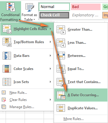
- To apply the formatting, you simply go to the Home tab > Conditional Formatting > Highlight Cell Rules and select A Date Occurring.
- Select one of the date options from the drop-down list in the left-hand part of the window, ranging from last month to next month.
- Finally, choose one of the pre-defined formats or set up your custom format by choosing different options on the Font, Border and Fill tabs. If the Excel standard palette does not suffice, you can always click the More colors… button.

- Click OK and enjoy the result! : )
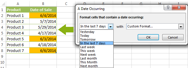
However, this fast and straightforward way has two significant limitations - 1) it works for selected cells only and 2) the conditional format is always applied based on the current date.
Excel conditional formatting formulas for dates
If you want to highlight cells or entire rows based on a date in another cell, or create rules for greater time intervals (i.e. more than a month from the current date), you will have to create your own conditional formatting rule based on a formula. Below you will find a few examples of my favorite Excel conditional formats for dates.
How to highlight weekends in Excel
Regrettably, Microsoft Excel does not have a built-in calendar similar to Outlook's. Well, let's see how you can create your own automated calendar with quite little effort.
When designing your Excel calendar, you can use the =DATE(year,month,date) function to display the days of the week. Simply enter the year and the month's number somewhere in your spreadsheet and reference those cells in the formula. Of course, you could type the numbers directly in the formula, but this is not a very efficient approach because you would have to adjust the formula for each month.
The screenshot below demonstrates the DATE function in action. I used the formula =DATE($B$2,$B$1,B$4) which is copied across row 5.

Tip. If you want to display only the days of the week like you see in the image above, select the cells with the formula (row 5 in our case), right-click and choose Format Cells…> Number > Custom. From the drop-down list under Type, select either dddd or ddd to show full day names or abbreviated names, respectively.
Your Excel calendar is almost done, and you only need to change the color of weekends. Naturally, you are not going to color the cells manually. We'll have Excel format the weekends automatically by creating a conditional formatting rule based on the WEEKDAY formula.
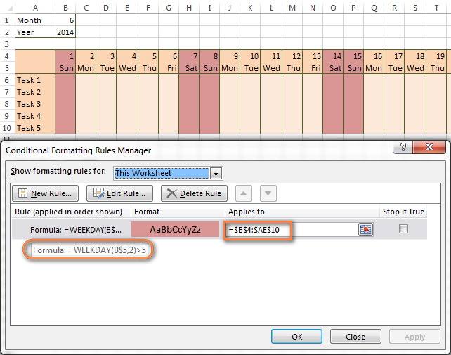
- You start by selecting your Excel calendar where you want to shade the weekends. In our case, it is the range $B$4:$AE$10. Be sure to start the selection with the 1st date column - Colum B in this example.
- On the Home tab, click Conditional Formatting menu > New Rule.
- Create a new conditional formatting rule based on a formula as explained in the above linked guide.
- In the "Format values where this formula is true" box, enter the following WEEKDAY formula that will determine which cells are Saturdays and Sundays:
=WEEKDAY(B$5,2)>5 - Click the Format… button and set up your custom format by switching between the Font, Border and Fill tabs and playing with different formatting options. When done, click the OK button to preview the rule.

Now, let me briefly explain the WEEKDAY(serial_number,[return_type]) formula so that you can quickly adjust it for your own spreadsheets.
- The
serial_numberparameter represents the date you are trying to find. You enter a reference to your first cell with a date, B$5 in our case. - The
[return_type]parameter determines the week type (square brackets imply it is optional). You enter 2 as the return type for a week starting from Monday (1) through Sunday (7). You can find the full list of available return types here. - Finally, you write >5 to highlight only Saturdays (6) and Sundays (7).
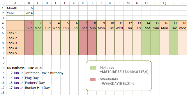
The screenshot below demonstrates the result in Excel 2013 - the weekends are highlighted in the reddish colour.
Tips:
- If you have non-standard weekends in your company, e.g. Fridays and Saturdays, then you would need to tweak the formula so that it starts counting from Sunday (1) and highlight days 6 (Friday) and 7 (Saturday) -
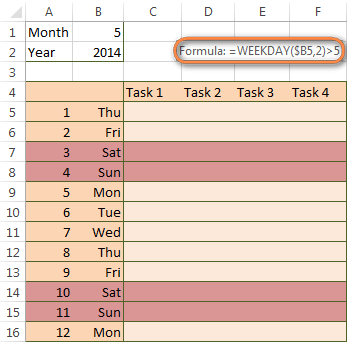
WEEKDAY(B$5,1)>5. - If you are creating a horizontal (landscape) calendar, use a relative column (without $) and absolute row (with $) in a cell reference because you should lock the reference of the row - in the above example it is row 5, so we entered B$5. But if you are designing a calendar in vertical orientation, you should do the opposite, i.e. use an absolute column and relative row, e.g. $B5 as you can see in the screenshot below:
How to highlight holidays in Excel
To improve your Excel calendar further, you can shade public holidays as well. To do that, you will need to list the holidays you want to highlight in the same or some other spreadsheet.
For example, I've added the following holidays in column A ($A$14:$A$17). Of course, not all of them are real public holidays, but they will do for demonstration purposes : )

Again, you open Conditional Formatting > New Rule. In the case of holidays, you are going to use either MATCH or COUNTIF function:
=COUNTIF($A$14:$A$17,B$5)>0=MATCH(B$5,$A$14:$A$17,0)
Note. If you have chosen a different color for holidays, you need to move the public holiday rule to the top of the rules list via Conditional Formatting > Manage Rules…
The following image shows the result in Excel 2013:
Conditionally format a cell when a value is changed to a date
It's not a big problem to conditionally format a cell when a date is added to that cell or any other cell in the same row as long as no other value type is allowed. In this case, you could simply use a formula to highlight non-blanks, as described in Excel conditional formulas for blanks and non-blanks. But what if those cells already have some values, e.g. text, and you want to change the background color when text is changed to a date?
The task may sound a bit intricate, but the solution is very simple.
- First off, you need to determine the format code of your date. Here are just a few examples:
- D1: dd-mmm-yy or d-mmm-yy
- D2: dd-mmm or d-mmm
- D3: mmm-yy
- D4: mm/dd/yy or m/d/yy or m/d/yy h:mm
You can find the complete list of date codes in this article.
- Select a column where you want to change the color of cells or the entire table in case you want to highlight rows.
- And now create a conditional formatting rule using a formula similar to this one:
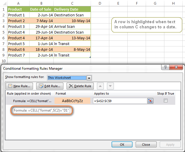
=CELL("format",$A2)="D1". In the formula, A is the column with dates and D1 is the date format.If your table contains dates in 2 or more formats, then use the OR operator, e.g.
=OR(cell("format", $A2)="D1", cell("format",$A2)="D2", cell("format", $A2)="D3")The screenshot below demonstrates the result of such conditional formatting rule for dates.
How to highlight rows based on a certain date in a certain column
Suppose, you have a large Excel spreadsheet that contains two date columns (B and C). You want to highlight every row that has a certain date, say 13-May-14, in column C.
To apply Excel conditional formatting to a certain date, you need to find its numerical value first. As you probably know, Microsoft Excel stores dates as sequential serial numbers, starting from January 1, 1900. So, 1-Jan-1900 is stored as 1, 2-Jan-1900 is stored as 2… and 13-May-14 as 41772.
To find the date's number, right-click the cell, select Format Cells > Number and choose the General format. Write down the number you see and click Cancel because you do not really want to change the date's format.

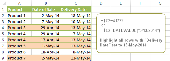
That was actually the major part of the work and now you only need to create a conditional formatting rule for the entire table with this very simple formula: =$C2=41772. The formula implies that your table has headers and row 2 is your first row with data.
An alternative way is to use the DATEVALUE formula that converts the date to the number format is which it is stored, e.g. =$C2=DATEVALUE("5/13/2014")
Whichever formula you use, it will have the same effect:
Conditionally format dates in Excel based on the current date
As you probably know Microsoft Excel provides the TODAY() functions for various calculations based on the current date. Here are just a few examples of how you can use it to conditionally format dates in Excel.
Example 1. Highlight dates equal to, greater than or less than today
To conditionally format cells or entire rows based on today's date, you use the TODAY function as follows:
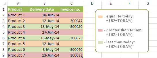
Equal to today: =$B2=TODAY()
Greater than today: =$B2>TODAY()
Less than today: =$B2<TODAY()
The screenshot below demonstrates the above rules in action. Please note, at the moment of writing TODAY was 12-Jun-2014.
Example 2. Conditionally format dates in Excel based on several conditions
In a similar fashion, you can use the TODAY function in combination with other Excel functions to handle more complex scenarios. For example, you may want your Excel conditional formatting date formula to color the Invoice column when the Delivery Date is equal to or greater than today BUT you want the formatting to disappear when you enter the invoice number.
For this task, you would need an additional column with the following formula (where E is your Delivery column and F the Invoice column):
=IF(E2>=TODAY(),IF(F2="", 1, 0), 0)
If the delivery date is greater than or equal to the current date and there is no number in the Invoice column, the formula returns 1, otherwise it's 0.
After that you create a simple conditional formatting rule for the Invoice column with the formula =$G2=1 where G is your additional column. Of course, you will be able to hide this column later.

Example 3. Highlight upcoming dates and delays
Suppose you have a project schedule in Excel that lists tasks, their start dates and durations. What you want is to have the end date for each task calculated automatically. An additional challenge is that the formula should also consider the weekends. For example, if the starting date is 13-Jun-2014 and the number of days of work (Duration) is 2, the ending date should come as 17-Jun-2014, because 14-Jun and 15-Jun are Saturday and Sunday.
To do this, we will use the WORKDAY.INTL(start_date,days,[weekend],[holidays]) function, more precisely =WORKDAY.INTL(B2,C2,1).
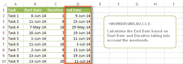
In the formula, we enter 1 as the 3rd parameter since it indicates Saturday and Sunday as holidays. You can use another value if your weekends are different, say, Fri and Sat. The full list of the weekend values is available here. Optionally, you can also use the 4th parameter [holidays], which is a set of dates (range of cells) that should be excluded from the working day calendar.
And finally, you may want to highlight rows depending on how far away the deadline is. For example, the conditional formatting rules based on the following 2 formulas highlight upcoming and recent end dates, respectively:
=AND($D2-TODAY()>=0,$D2-TODAY()<=7)- highlight all rows where the End Date (column D) is within the next 7 days. This formula is really handy when it comes to tracking upcoming expiration dates or payments.=AND(TODAY()-$D2>=0,TODAY()-$D2<=7)- highlight all rows where the End Date (column D) is within the last 7 days. You can use this formula to track the latest overdue payments and other delays.
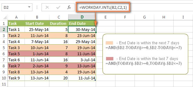
Here are a few more formula examples that can be applied to the table above:
=$D2<TODAY() - highlights all passed dates (i.e. dates less than the current date). Can be used to format expired subscriptions, overdue payments etc.
=$D2>TODAY() - highlights all future dates (i.e. dates greater than the current date). You can use it to highlight upcoming events.
Of course, there can be infinite variations of the above formulas, depending on your particular task. For instance:
=$D2-TODAY()>=6 - highlights dates that occur in 6 or more days.
=$D2=TODAY()-14 - highlights dates occurring exactly 2 weeks ago.
How to highlight dates within a date range
If you have a long list of dates in your worksheet, you may also want to highlight the cells or rows that fall within a certain date range, i.e. highlight all dates that are between two given dates.
You can fulfil this task using the TODAY() function again. You will just have to construct a little bit more elaborate formulas as demonstrated in the examples below.
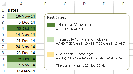
Formulas to highlight past dates
- More than 30 days ago:
=TODAY()-$A2>30 - From 30 to 15 days ago, inclusive:
=AND(TODAY()-$A2>=15, TODAY()-$A2<=30) - Less than 15 days ago:
=AND(TODAY()-$A2>=1, TODAY()-$A2<15)
The current date and any future dates are not colored.
Formulas to highlight future dates
- Will occur in more than 30 days from now:
=$A2-TODAY()>30 - In 30 to 15 days, inclusive:
=AND($A2-TODAY()>=15, $A2-TODAY()<=30) - In less than 15 days:
=AND($A2-TODAY()>=1, $A2-TODAY()<15)
The current date and any past dates are not colored.

How to shade gaps and time intervals
In this last example, we are going to utilize yet another Excel date function - DATEDIF(start_date, end_date, interval). This function calculates the difference between two dates based on the specified interval. It differs from all other functions we've discussed in this tutorial in the way that it lets you ignore months or years and calculate the difference only between days or months, whichever you choose.
Don't see how this could work for you? Think about it in another way… Suppose you have a list of birthdays of your family members and friends. Would you like to know how many days there are until their next birthday? Moreover, how many days exactly are left until your wedding anniversary and other events you wouldn't want to miss? Easily!
The formula you need is this (where A is your Date column):
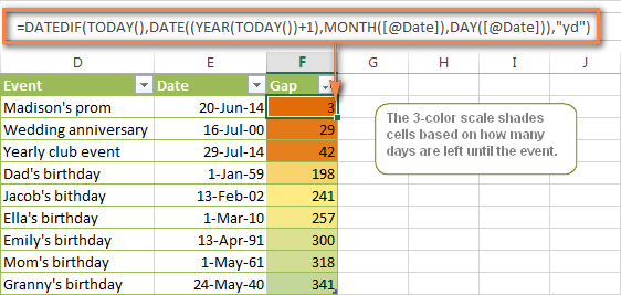
=DATEDIF(TODAY(), DATE((YEAR(TODAY())+1), MONTH($A2), DAY($A2)), "yd")
The "yd" interval type at the end of the formula is used to ignore years and calculate the difference between the days only. For the full list of available interval types, look here.
Tip. If you happen to forget or misplace that complex formula, you can use this simple one instead: =365-DATEDIF($A2,TODAY(),"yd"). It produces exactly the same results, just remember to replace 365 with 366 in leap years : )
And now let's create an Excel conditional formatting rule to shade different gaps in different colors. In this case, it makes more sense to utilize Excel Color Scales rather than create a separate rule for each period.
The screenshot below demonstrates the result in Excel - a gradient 3-color scale with tints from green to red through yellow.
"Days Until Next Birthday" Excel Web App
We have created this Excel Web App to show you the above formula in action. Just enter your events in 1st column and change the corresponding dates in the 2nd column to experiment with the result.
If you are curious to know how to create such interactive Excel spreadsheets, check out this article on how to make web-based Excel spreadsheets.
Hopefully, at least one of the Excel conditional formats for dates discussed in this article has proven useful to you. If you are looking for a solution to some different task, you are most welcome to post a comment. Thank you for reading!
 by
by
1200 comments
Hi, I have a training spreadsheet which shows a date in cells to show when training was completed. I would like a formula which changes these cells to a colour when they are due for renewal in 3 years time. Some cells are blank which shows training hasn't been completed, so these cells will need to be the same colour as above. Thank you for your help.
Hi Sarah,
You can use one of the following formulas in your conditional formatting rule:
=AND($C1<>"",Today()-$C1>=365*3)
or
=AND($C1<>"",DATEDIF($C1, TODAY(),"y")>=3)
Here C is the column with the training dates.
You can see this blog post for more details about calculating date differences:
https://www.ablebits.com/office-addins-blog/excel-datedif-calculate-date-difference/#count-days-between-dates
Can you help me? I want to use conditional formatting where the cell is to be green if that date (from another cell) is under 14 days and will input the 14th day. Then the cell is colored red if over 14 days.
Example: 1/7/16 IN ANOTHER CELL(in green) 1/21/16
12/15/16 (in red) (blank)
Hello Beve,
You can create two rules with the following formulas:
1) Apply green color if the date in cell B2 is not more than 14 days away from the date in cell A2:
=AND(ABS(INT(B2-A2))<=14,NOT(ISBLANK(B2)))
2) Apply red if the date in cell C2 is over 14 days away from the date in A2:
=AND(ABS(INT(C2-A2))>14,NOT(ISBLANK(C2)))
These rules ignore blanks.
Is it possible to condition a single cell to change colors based on its entered date vs. the current date? As an example using a cell with a Due Date, I want the cell to stay "green" up to 3-days before it is due. At the 3-day mark turn "yellow". After the 3rd day and it passes its original due date it turns "red".
Any assistance would be much appreciated-JM
Hello James,
You can create three separate conditional formatting rules using the formulas below:
- One rule will apply green color when there are more than 3 days left:
=C2-B2>3
One rule is for turning cells yellow if there are 3 days left to the due date:
=C2-B2=3
The third rule will highlight the cells red when there are fewer than 3 days to the due date and 3 days after it:
=AND(C2-B2<3,C2-B2>-3)
Here C2 is the due date, and B2 is the cell with the current date.
HI,
I WANT TO CALCULATE HOW MANY DAYS THERE ARE UNTIL THE NEXT RENEWAL FOR THEIR VISA. AM CREATING A EMPLOYEE DATABASE.
=DATEDIF(TODAY(),DATE((YEAR(TODAY())+1),MONTH($A2),DAY($A2)),"yd")
I TRIED THIS AND WORKING FINE. BUT I NEED IT FOR 2-4 YEARS CALCULATION.
Hello Saj,
You need to replace the "yd" parameter in your formula with "d".
Please suggest how to highlight 2nd and 4th Sat and all Sunday in a month as weekend using conditional formatting.
Hello Mali,
You can create separate rules to highlight certain days of the week. You can use the following formula for the rule that highlights Sundays:
=WEEKDAY(A2)=1
You can use the following formula to highlight the second Saturday each month:
=(DATE(YEAR(A2),MONTH(A2),1)+(7-WEEKDAY(DATE(YEAR(A2),MONTH(A2),1)))+7)=A2
Here is the formula for highlighting every 4th Saturday:
=(DATE(YEAR(A2),MONTH(A2),1)+(7-WEEKDAY(DATE(YEAR(A2),MONTH(A2),1)))+21)=A2
Hi SVetlana
I need solution to highlight 2nd and 4th Saturday and all Sundays in a month. I am not expert in excel. Please advise.
Mali
I am trying to color code a date in a column if the date in the column is < or = to the date in the column before it.
Example if the date in Column G is <or= to date in Column F color the cell green.
Every formula I have tried so far has not give me the results I am looking for.
=IF(f<=g,TRUE,FALSE) =IFdate(G<=F,true, false) =if date g<=f
I am using exel version 2013 and use a formula to determine which cells to format under the new formatting rules.
Any assistance would be greatly appreciate. Thank you,
Hello Bonny,
You can use the following simple formula for your conditional formatting rule:
=F2<=G2
If there are blanks in the range, you can ignore them by using this formula instead:
=AND(NOT(ISBLANK(G2)),F2<=G2)
Hi Svetlana,
I am using Excel 2003 and I am trying to change cells in column B red if the date is 6 weeks greater than the date in column B. I am not sure how to get excel to recongise this other than today.
Thanks
Hi Svetlana,
we have created sheet for Service report tracker to my team, so if some one log a complaint today that compliant it should show one colour if still the complaint not fixed it in 15 days it has to go to different colour and if the compliant call has closed it has to go to the different colour Can you tell me the formula I should use?
Hi Peter,
You need to create two conditional formatting rules and choose to use the formulas below. Say, if your dates are in column A, and a note that the complaint is fixed is in column B, then use one rule to highlight all dates in column A red if more than 15 days passed and if the cell in column B is blank:
=AND(TODAY()-A2>15,ISBLANK(B2),NOT(ISBLANK(A2)))
Create the second rule to highlight cells in column A green if there is anything entered in column B:
=AND(NOT(ISBLANK(B2)),NOT(ISBLANK(A2)))
created a timesheet for employees that highlights weekends and Federal Holidays. would like a formula for conditional formatting to highlight the Federal holiday a day before or a day after if it falls on a weekend. e.g. 4th of July 2015 falls on Saturday, instead of highlighting that Saturday, want to highlight the day before Saturday(in this case Friday July 3). If it had fallen on Sunday, i'd like to highlight the next day(in this case Monday). thanks,
Hi, i am trying to format - highlight a rows based on date in the corresponding cell in that row, so every day would the row would have a different color.
For example i have a table :
A1 - Task column, B1- Date, C3 - Start time, D4 - End time and etc.
so it might be several tasks different rows following one after another for 11/25/2015
so i it can be only two colors but need to highlight all rows for that day in one color and let say - next day 11/26/2015 i have more tasks to be highlighted in another color.
I would really appreciate your help, thanks
Hello Andrey,
You can alternate row colors when the date changes, please see the solution described here:
https://www.ablebits.com/office-addins-blog/alternate-row-colors-excel/#value-based
If you want to use more colors, you can create conditional formatting rules for as many colors as you want to use with the formulas below. Say, if you want to use 3 colors, you would need to create three rules with the following formulas and assign each one a color:
=MOD($B2,3)=2
=MOD($B2,3)=1
=MOD($B2,3)=0
Hi I am trying to show various cells at different stages from an expiration date! So if Colum E is 31/12/2015. i would like blank cells within L-S to show once they are say L is 15 days past this and M 3mths past this and N is 6 mths past this etc? Is this possible??
Thanks in advance?
Hello Gareth,
If we understand your task correctly, you can create conditional formatting rules with formulas for each of the cells you want to highlight, e.g. for M4 the formula would be:
=E4-D4<=90
Here E4 is the cell with the expiration date and D4 is the cell with the current date. If
You can add another rule for N4 the same way:
=E4-D4<=180
Hi Svetlana,
I have a member roster where dues expire at the end of the year. They are entered as 2015/12/31 in column S beginning in row 3.
I need two formulas. Because the member's name is far to the left in column A, I want to (1) change the cell fill color of the member name if the expiration date is in the current year and (2) if the expiration date is in the previous year or earlier. I want to apply the formula to all rows of members, more than 500 names.
Would you help me? How could I do that with conditional formatting?
Many thanks and looking forward to your help.
Hello Joe,
You need to create two conditional formatting rules with the option to "Use a formula to determine which cells to format", and apply the rules to column A.
One rule should look for years that are earlier than the current:
=YEAR(S3)<YEAR(TODAY())
The second rule should find the current year:
=YEAR(S3)=YEAR(TODAY())
Hello Swetlena,
Is there any way in which I can use Red & Green coloue together in one column to reflect the expiry date.
The green colour fades more towards the red colour as the expiry date approaches?
Regards,
Akhil
Hello Akhil,
You can select the range with dates and create a conditional formatting rule with the "2-Color Scale" format style. Select green color for the minimum value and red for the maximum value, choose to use formula for the maximum value and refer to the cell with the expiry date, e.g. =$B$11.
Hi Miss Svetlana,
I have a problem on my report. My Boss want to see the my data and highlighted using conditional formatting for the clients have no record or data for past six months and my report was format by month. I hope you can help on this.
Thank you.
Hello Adrian,
When you create a conditional formatting rule, choose to "Use a formula to determine which cells to format" and try the following formula:
=A2>EOMONTH(TODAY()-210,0)+1
I have a problem with conditional formatting "greater than value".
I'm trying to create a new rule wherein the values are results of time difference and of "if" formula.
This is how it goes. =if((7:05 AM-7:00 AM)>0,(7:05 AM-7:00 AM),"0:00) but the formula bar contains =if((K11-M11)>0,M11-K11,"0:00")
The answer should be 0:05 mins and I tried conditional formatting it.
The conditional formatting rule is like this;"Cell Value>0:00","AaBbCc"(this are formatted in red font color),Applies to cells from "=$O$11:$O$16".
The answer in from the formula bar should turn red(0:05) and it did, except the problem is it turned all the other cells answers (0:00) into red.
Hello,
You can use a simple formula =M11-K11 first and set the cell format to time -> 13:30. This way you will see minutes in the format you need. Then create a conditional formatting rule based on the following formula:
=MINUTE(M3-K3)>4
It will highlight all values that are over 4 minutes.
Hi Svetlana
If training dates are entered within a range of cells for the current month (if we are in Oct, then all dates will be October dates), and all cells are formatted so that dates entered are red and look like dd/mm/yyyy, how can I conditionally format the red dates for October to change to black 5 days into the new month so that any new November dates entered at the start of the month remain red, while the rest change?
Essentially, we need a gap between the end of the month and when the previous month's dates change so that we can send reports of previous month's activities.
Would really appreciate your help with this.
Thanks :)
Hello Lynette,
Please try to create a new conditional formatting rule, choose to "Use a formula to determine which cells to format" and enter the following formula:
=OR(MONTH(A2)=1, A2<=EOMONTH($A$2,0)+5)
Please replace column A with the column where you have the dates.
Click "Format" to change the found dates to black font and click Ok.
Hi, I have random dates of the year in a column now I want to highlight the higher/last date of each month but not able to find any condition need help.
Ex-
8-Feb-15
9-Feb-15
10-Feb-15
20-Apr-15 (Highlight this)
1-Mar-15
2-Mar-15
10-Mar-15 (Highlight this)
17-Apr-15
18-Apr-15
1-May-15
5-May-15
6-May-15
8-May-15
9-May-15 (Highlight this)
10-Jan-15
11-Jan-15
24-Jan-15
25-Jan-15
26-Jan-15 (Highlight this)
8-Feb-15
11-Feb-15
24-Feb-15
25-Feb-15 (Highlight this)
Hello Bhardwaj,
You need to create a conditional formatting rule, choose to "Use a formula to determine which cells to format" and enter the following formula:
=IF(C2<>"",LOOKUP(2,1/(C2-DAY(C2)=C$2:C$100-DAY(C$2:C$100)),C$2:C$100)=C2,FALSE)
Here C2:C100 is the range with your dates.
Select format for the cells and click Ok.
I need to calculate the days between a start date (A1) and today but to stop calculating when an end date is entered in cell (A2) so (A3) will show how many days have passed but when I open the file after the end date I don't want the calculation to continue going forward.
Hello Dale,
Please try one of the following formulas in A3 to calculate the number of days between the start date and today, or between the start day and the end date if it is entered in cell A2:
=IF(A2="";TODAY()-A1; A2-A1)
Or
=IF(ISBLANK(A2); TODAY()-A1;A2-A1)
HI,
HOw to print the current date in a cell based upon the change in the color of the cell?
Hello Pruthi,
If we understand your task correctly, you can use the following VBA code that one of our developers wrote for you:
- Open your Excel file;
- Press Alt+F11 on your keyboard;
- Double-click the sheet name in the list and paste the code below, but change the reference to your data range and the cell with the necessary color:
Private Sub CommandButton1_Click()
Dim color
Dim i As Integer
Range("J2").Select
color = Selection.Interior.color
Range("F2:F11").Select
For i = 2 To 11
Range("F" & i).Select
If Selection.Interior.color = color Then
Selection.Value = Date
End If
Range("G" & i).Select
If Selection.Interior.color = color Then
Selection.Value = Date
End If
Next i
End Sub
- Click Run
Hi Svetlana,
I want to use conditional formatting to show (via color highlighting) if a date entered into a cell is within the current calendar year (at any time the spreadsheet is opened). Can you tell me the formula I should use?
Thanks!
Hi Kevin,
You can create an Excel conditional formatting rule based on a formula similar to this:
=YEAR(TODAY())=YEAR($A1)
Where A1 is the cell containing your date.
Hi I am a total loss here
I have a column (D5) with Certificate Test/Start dates (YYYY/MM/DD) I then have a column (E5) with months eg. 3,6,12,24 etc, these indicate the months before the certificate needs to be "retested".
These month values are variables so I can't hardcode a value like Cell Value less than =NOW()-365 (This is for a year validity certificate) and =NOW()-(E5*30.5) meaning month x days, this doesn't work or I am just screwing up the format.
I want to do a conditional format on D5 that uses E5 to flag D5 as RED (expired), YELLOW (30 days before expiry) and GREEN (still valid)
Can anyone please help :(
Hi Nick,
You can use the following formula to calculate the expiry dates:
=DATE(YEAR($D5), MONTH($D5)+$E5, DAY($D5))
And than you can create 3 rules with the following formulas based on the expiry date (say in column G):
Red:=$G5-TODAY()>30
Yellow:=AND($G5>TODAY(),$G5-TODAY()<=30)
Green: =$G5-TODAY()>30
If you don't want an additional column with expiry dates, you can replace G5 in the conditional formatting formulas with the Date function, e.g.:
Green: =DATE(YEAR($D5), MONTH($D5)+$E5, DAY($D5))-TODAY()>30
Hi,
I have a date, order #, and arrival date columns
is there a way to highlight the arrival date column if it is empty after 24 hours from the respective order date?
For Example:
order # 3 is placed on 10/04/15 and arrival date is not mentioned until 10/06/15 then it should be highlighted in a different color on 10/05/15
Hello Lijina,
Supposing that the order date is in column A and arrival date is in column B, and row 2 is the topmost row with dates, select the arrival date column (B) beginning with row 2, and create a rule with the following formula:
=AND(TODAY()-($A2+1)>0, $B2="", $A2<>"")
Hello,
I want to highlight an entire row in which only one cell (H2) contains a date. I would like my whole row to be highlighted red when the date in this cell(H5)is two days away from today (coming up in 2 days).
Thank you very much
H2 again sorry, not H5
Hello Nicolas,
Select the entire rows that you want to highlight beginning with your first row with dates, e.g. A2:I100. And create a rule with one of the following formulas:
Date in H2 is exactly two days away from today:
=$H2-TODAY()=2
Date in H2 is 1 or 2 days away from today:
=AND($H2-TODAY()>0, $H2-TODAY()<=2)
Hi,
I am trying to format cells so that if one date is entered it will be yellow, if two dates are entered it will become orange and if three dates are entered it will become green. Dates (Uk style! :)) will be all listed in the same cell either:
- dd/mm/yy (yellow)
- dd/mm/yy, dd/mm/yy (orange)
- dd/mm/yy, dd/mm/yy, dd/mm/yy (green)
Do you know if this is possible please and do you have any tips on achieving this?
Many thanks in advance!
Hi Georgie,
Because two or more dates entered in the same cell turn into a usual text string, you can write formulas based on how many commas a certain cell contains, if any.
For example, if your dates reside in column A beginning in row 2, you can use the following formulas:
Green (3 dates): =SEARCH(",*,", $A2)
Orange (2 dates): =SEARCH(",", $A2)
Yellow (1 date): =$A2<>""
Please note, the rules order is important, so make sure the green rule is the first in the list of rule, and the yellow rule is the last.
It was very useful using your tips..
Thank you..
I have a date column to identify when individuals leave. I would like the color to change from green being >90 days out, <90 days out- yellow, and <30 days out red. How do I accomplish this?
Hello Caleb,
Please check out the following tutorial that dwells on conditional formatting for dates:
https://www.ablebits.com/office-addins-blog/excel-conditional-formatting-dates/
order date un/st back order estimated arrival
12 21/9/15 unit yes
13 21/9/15 stock no
14 22/9/15 stock yes 24/09/15
15 23/9/15 unit no
estimated arrival time column is conditional formatted with =AND(c2="unit down", d2="yes", ISBLANK(e2))
which is if the order is unit and back order is yes and estimated arrival time is not mentioned then it highlights in red.
is there a way I could also add a condition with the above mentioned one...which will also highlight in red if the estimated time is not filled even after 24 hours from the date the order has been placed (column B)?
Hi, I have random dates of the year in a column now I want to highlight the higher/last date of each month but not able to find any condition need help.
Ex-
8-Feb-15
9-Feb-15
10-Feb-15
20-Apr-15 (Highlight this)
1-Mar-15
2-Mar-15
10-Mar-15 (Highlight this)
17-Apr-15
18-Apr-15
1-May-15
5-May-15
6-May-15
8-May-15
9-May-15 (Highlight this)
10-Jan-15
11-Jan-15
24-Jan-15
25-Jan-15
26-Jan-15 (Highlight this)
8-Feb-15
11-Feb-15
24-Feb-15
25-Feb-15 (Highlight this)
Hello, I am employed as a Training coordinator and am trying to have cells in excel turn yellow when an employees' certification is within 30 days of expiry. And then turn red when the certification is expired.
This is based off a certification that is valid for a 3 year duration.
Any help with this would be greatly appreciated.
Hi,
I would like to set up 4 columns that change colour based on the date in the another column.
E.G if column E is the 1/5/15 I would like column F to turn yellow 30 days after the 1st then Red 10 days after that.
Once a date is entered in column F I would like G to turn yellow 30 days later and red another 10 days after that.
once a date is entered in column G I would like H to turn yellow 30 days later and red 10 days after that.
Once a date is in H column I would like I to turn yellow 30 days later and red 10 days after that.
Your help is much appreciated.
Please correct if condition formula.
=IF(H2<"6:00:00","Standard",IF(H2<"8:00:00","Prime",IF(H2<"10:00:00","Standard",IF(H2<"18:00:00","Prime",IF(H2<"20:00:00","Standard",IF(H2<"22:00:00","Lean","Error"))))))
how to separate particulars time format data. i want to use if condition formula. please reply formula in my e-mail ID.
Exm.
10:00:00 AM to 18:00:00 PM (Standard Time)
18:00:01 PM to 22:00:00 PM (Lean Time)
Data
01:00:00
02:00:00
03:00:00
04:00:00
05:00:00
06:00:00
07:00:00
08:00:00
09:00:00
10:00:00
11:00:00
12:00:00
13:00:00
14:00:00
15:00:00
16:00:00
17:00:00
18:00:00
19:00:00
20:00:00
21:00:00
22:00:00
23:00:00
00:00:00
10:00:00 AM to 18:00:00 PM (Standard Time)
18:00:01 PM to 22:00:00 PM (Lean Time)
Hi, I have a list of persons with their birthdates.
I need to check only on a certain month.
For example: if the birthdate is in October of any year, I need to take an action.
For any other birthdate, no specific action is needed.
Therefore I want to conditionally format with a color so I can filter or sort on the color.
Thanks for your cooperation.
Can I apply 2 conditional formats to the one cell such as:
1.If the cell value changes from $0.00 to a higher amount the text colour will change to red, this conditional formatting I have successfully set.
2. the text colour of the same cell as above will change to blue if the date changes to a date in the current month in another cell? I have tried a few different formulas, nothing seems to work.
Hi, I have random dates of the year in a column now I want to highlight the higher/last date of each month but not able to find any condition need help.
Ex-
8-Feb-15
9-Feb-15
10-Feb-15
20-Apr-15 20-Apr-15
1-Mar-15
2-Mar-15
10-Mar-15 10-Mar-15
17-Apr-15
18-Apr-15
1-May-15
5-May-15
6-May-15
8-May-15
9-May-15 9-May-15
10-Jan-15
11-Jan-15
24-Jan-15
25-Jan-15
26-Jan-15 26-Jan-15
8-Feb-15
11-Feb-15
24-Feb-15
25-Feb-15 26-Feb-15
Hi. I am trying to create a tracker for all employee certificates. Columns represent each employee and rows define the dates of expiry of certificates. I would like to change the color of the cells when the expiry date is getting closer to today's date. Orange for dates within 15-30 days, red orange for 0-14 days and red for expired dates. I also want to highlight in green the valid dates. I have tried doing it using the formula below but when I test it, the whole row becomes orange and not just the cell. I don't know what I am doing wrong. Please help. Thanks.
=AND($A$2-TODAY()>15,$A$2-TODAY()<=30)
I use template Pro, I need help this.
Saturday and Sunday are excluded from workday in Gantt chart pro, but I want to exclude only Sunday. How can I changed this?
how to calculate number of days less than 1 month from column with dates. I couldn't find a formula for this. Is it so simple as it is not here?
Hi Monica,
If you want to highlight the past dates within 1 month from today's date, you can create a rule with the following formula:
=TODAY()-$A2<=30
If you are looking for something different, please clarify.
Also, not sure if this matters but I applied it to rows instead of columns and that seemed to help as well.
SOLVED IT!! This formula works! Posting in case someone else needs it. :-)
=AND($E2<DATEVALUE("2/7/2015"), $F2<DATEVALUE("2/7/2015"))
Second formula: =AND($E2>DATEVALUE("2/7/2015"), $F2>DATEVALUE("2/7/2015"))
It just keeps combinging my formulas....trying two separate comments.
First formula: =AND(42041<$E2, 42041<$F2)
Not sure what happened with my first comment but it combined my formulas together. The first one I tried was: =AND(42041<$E2, 42041DATEVALUE("2/7/2015"), $F2>DATEVALUE("2/7/2015"))
I need help with the following issue. I have a spreadsheet with two columns that contain dates and times in this format: 02/06/2015 12:00AM. All of the cells in column E have values but some of the cells in column F are blank. What I need is for columns A-D to be conditionally formatted when the value of column E AND column F occur before 2/6/2015. I have tried these formulas and they both work on some rows but not on all rows and I cannot figure out why.
First formula I tried: =AND(42041<$E2, 42041DATEVALUE("2/7/2015"), $F2>DATEVALUE("2/7/2015"))
Both of the above formulas will conditionally format some rows correctly but they both also conditionally format some rows incorrectly and I cannot figure out why Excel can calculate the formula correctly sometimes but not other times. There is no difference in the data types between the rows where the formulas work and the formulas do not work.
Any help is greatly appreciated.
Just needed some help with conditional formatting. I have two columns both with dates - Column A and B. I want to highlight only the dates in B which Date occur 10 days after the date of Column A
Hi Alwin,
You can create a rule with the formula =$B2-$A2=10 (row 2 is supposed to be the first row with data.
Thanks for your reply
while I am using this formula it is showing TRUE/FALSE. Actually I need to highlight that column with a specific color and also need to see the date.
I need to highlight the Column B.
To highlight the column, you need to create a conditional formatting rule with the above formulas. You can find the detailed steps to create a rule in this tutorial.
Hi Svetlana Cheusheva,
Still I am unable to do this. Please help me to highlight the column B
Column A Column B
01-04-2015 11-04-2015
02-04-2015 17-04-2015
03-04-2015 23-04-2015
04-04-2015 09-04-2015
05-04-2015 15-04-2015
06-04-2015 21-04-2015
07-04-2015 27-04-2015
08-04-2015 13-04-2015
09-04-2015 19-04-2015
10-04-2015 25-04-2015
11-04-2015 01-05-2015
12-04-2015 17-04-2015
13-04-2015 23-04-2015
14-04-2015 29-04-2015
15-04-2015 05-05-2015
16-04-2015 21-04-2015
I need to be able to enter a date and then calculate backwards counting only school days. Example: field trip is October 1, 2015. Field trip packet is due 30 school days prior to trip. I need to exclude weekends, holidays and non-student days.
HI,
I have been trying to figure out a formula that changes the color of the cell to red if the date in the cell is <=10 days away from today's date. i.e if the date in the cell reads 07/12/2015 and I opened the spreed sheet today 07/22/2015 the date on that cell should be highlighted in red.
Hi Manny,
You can create a rule with the following formula, where A2 is the top-most cell with your dates:
=TODAY()-$A2>=10
Good day,
I have a column with dates and I need them to be highlighted if they do not fall in given windows.
For example:
Window 1: 1-May-15 till 12-Jun-15
Window 2: 26-Jun-15 till 31-Jul-15
Window 3: 14-Aug-15 till 18-Sep-15
Window 4: 2-Oct-15 till 6-Nov-15
So I need to know if 07/22/15 does not fall in between any of these windows and have it highlighted if it does not.
Thank you for your consideration.
Hi,
I'm trying to highlight a row depending on the difference in 2 dates.
e.g. if the difference is greater than 1 month then the row needs to go red, if less than a month then the row needs to go green.
Is there a formula that can do this?