If you are a regular visitor of this blog, you've probably noticed a few articles covering different aspects of Excel conditional formatting. And now we will leverage this knowledge and create spreadsheets that differentiate between weekdays and weekends, highlight public holidays and display a coming deadline or delay. In other words, we are going to apply Excel conditional formatting to dates.
If you have some basic knowledge of Excel formulas, then you are most likely familiar with some of date and time functions such as NOW, TODAY, DATE, WEEKDAY, etc. In this tutorial, we are going to take this functionality a step further to conditionally format Excel dates in the way you want.
Excel conditional formatting for dates (built-in rules)
Microsoft Excel provides 10 options to format selected cells based on the current date.
- To apply the formatting, you simply go to the Home tab > Conditional Formatting > Highlight Cell Rules and select A Date Occurring.
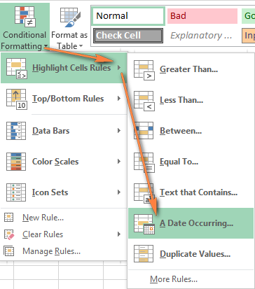
- Select one of the date options from the drop-down list in the left-hand part of the window, ranging from last month to next month.
- Finally, choose one of the pre-defined formats or set up your custom format by choosing different options on the Font, Border and Fill tabs. If the Excel standard palette does not suffice, you can always click the More colors… button.

- Click OK and enjoy the result! : )
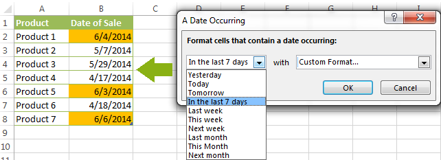
However, this fast and straightforward way has two significant limitations - 1) it works for selected cells only and 2) the conditional format is always applied based on the current date.
Excel conditional formatting formulas for dates
If you want to highlight cells or entire rows based on a date in another cell, or create rules for greater time intervals (i.e. more than a month from the current date), you will have to create your own conditional formatting rule based on a formula. Below you will find a few examples of my favorite Excel conditional formats for dates.
How to highlight weekends in Excel
Regrettably, Microsoft Excel does not have a built-in calendar similar to Outlook's. Well, let's see how you can create your own automated calendar with quite little effort.
When designing your Excel calendar, you can use the =DATE(year,month,date) function to display the days of the week. Simply enter the year and the month's number somewhere in your spreadsheet and reference those cells in the formula. Of course, you could type the numbers directly in the formula, but this is not a very efficient approach because you would have to adjust the formula for each month.
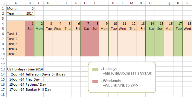
The screenshot below demonstrates the DATE function in action. I used the formula =DATE($B$2,$B$1,B$4) which is copied across row 5.

Tip. If you want to display only the days of the week like you see in the image above, select the cells with the formula (row 5 in our case), right-click and choose Format Cells…> Number > Custom. From the drop-down list under Type, select either dddd or ddd to show full day names or abbreviated names, respectively.
Your Excel calendar is almost done, and you only need to change the color of weekends. Naturally, you are not going to color the cells manually. We'll have Excel format the weekends automatically by creating a conditional formatting rule based on the WEEKDAY formula.
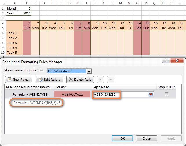
- You start by selecting your Excel calendar where you want to shade the weekends. In our case, it is the range $B$4:$AE$10. Be sure to start the selection with the 1st date column - Colum B in this example.
- On the Home tab, click Conditional Formatting menu > New Rule.
- Create a new conditional formatting rule based on a formula as explained in the above linked guide.
- In the "Format values where this formula is true" box, enter the following WEEKDAY formula that will determine which cells are Saturdays and Sundays:
=WEEKDAY(B$5,2)>5 - Click the Format… button and set up your custom format by switching between the Font, Border and Fill tabs and playing with different formatting options. When done, click the OK button to preview the rule.

Now, let me briefly explain the WEEKDAY(serial_number,[return_type]) formula so that you can quickly adjust it for your own spreadsheets.
- The
serial_numberparameter represents the date you are trying to find. You enter a reference to your first cell with a date, B$5 in our case. - The
[return_type]parameter determines the week type (square brackets imply it is optional). You enter 2 as the return type for a week starting from Monday (1) through Sunday (7). You can find the full list of available return types here. - Finally, you write >5 to highlight only Saturdays (6) and Sundays (7).
The screenshot below demonstrates the result in Excel 2013 - the weekends are highlighted in the reddish colour.
Tips:
- If you have non-standard weekends in your company, e.g. Fridays and Saturdays, then you would need to tweak the formula so that it starts counting from Sunday (1) and highlight days 6 (Friday) and 7 (Saturday) -
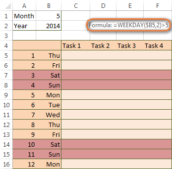
WEEKDAY(B$5,1)>5. - If you are creating a horizontal (landscape) calendar, use a relative column (without $) and absolute row (with $) in a cell reference because you should lock the reference of the row - in the above example it is row 5, so we entered B$5. But if you are designing a calendar in vertical orientation, you should do the opposite, i.e. use an absolute column and relative row, e.g. $B5 as you can see in the screenshot below:
How to highlight holidays in Excel
To improve your Excel calendar further, you can shade public holidays as well. To do that, you will need to list the holidays you want to highlight in the same or some other spreadsheet.
For example, I've added the following holidays in column A ($A$14:$A$17). Of course, not all of them are real public holidays, but they will do for demonstration purposes : )

Again, you open Conditional Formatting > New Rule. In the case of holidays, you are going to use either MATCH or COUNTIF function:
=COUNTIF($A$14:$A$17,B$5)>0=MATCH(B$5,$A$14:$A$17,0)
Note. If you have chosen a different color for holidays, you need to move the public holiday rule to the top of the rules list via Conditional Formatting > Manage Rules…
The following image shows the result in Excel 2013:
Conditionally format a cell when a value is changed to a date
It's not a big problem to conditionally format a cell when a date is added to that cell or any other cell in the same row as long as no other value type is allowed. In this case, you could simply use a formula to highlight non-blanks, as described in Excel conditional formulas for blanks and non-blanks. But what if those cells already have some values, e.g. text, and you want to change the background color when text is changed to a date?
The task may sound a bit intricate, but the solution is very simple.
- First off, you need to determine the format code of your date. Here are just a few examples:
- D1: dd-mmm-yy or d-mmm-yy
- D2: dd-mmm or d-mmm
- D3: mmm-yy
- D4: mm/dd/yy or m/d/yy or m/d/yy h:mm
You can find the complete list of date codes in this article.
- Select a column where you want to change the color of cells or the entire table in case you want to highlight rows.
- And now create a conditional formatting rule using a formula similar to this one:
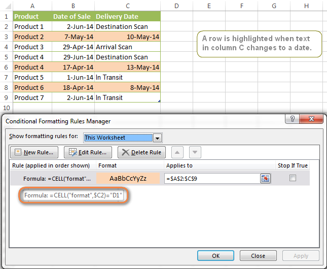
=CELL("format",$A2)="D1". In the formula, A is the column with dates and D1 is the date format.If your table contains dates in 2 or more formats, then use the OR operator, e.g.
=OR(cell("format", $A2)="D1", cell("format",$A2)="D2", cell("format", $A2)="D3")The screenshot below demonstrates the result of such conditional formatting rule for dates.
How to highlight rows based on a certain date in a certain column
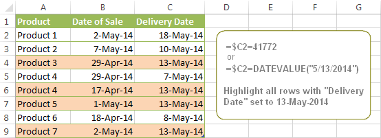
Suppose, you have a large Excel spreadsheet that contains two date columns (B and C). You want to highlight every row that has a certain date, say 13-May-14, in column C.
To apply Excel conditional formatting to a certain date, you need to find its numerical value first. As you probably know, Microsoft Excel stores dates as sequential serial numbers, starting from January 1, 1900. So, 1-Jan-1900 is stored as 1, 2-Jan-1900 is stored as 2… and 13-May-14 as 41772.
To find the date's number, right-click the cell, select Format Cells > Number and choose the General format. Write down the number you see and click Cancel because you do not really want to change the date's format.

That was actually the major part of the work and now you only need to create a conditional formatting rule for the entire table with this very simple formula: =$C2=41772. The formula implies that your table has headers and row 2 is your first row with data.
An alternative way is to use the DATEVALUE formula that converts the date to the number format is which it is stored, e.g. =$C2=DATEVALUE("5/13/2014")
Whichever formula you use, it will have the same effect:
Conditionally format dates in Excel based on the current date
As you probably know Microsoft Excel provides the TODAY() functions for various calculations based on the current date. Here are just a few examples of how you can use it to conditionally format dates in Excel.
Example 1. Highlight dates equal to, greater than or less than today
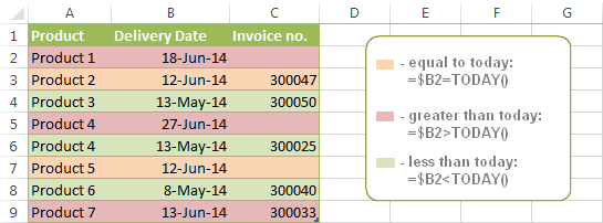
To conditionally format cells or entire rows based on today's date, you use the TODAY function as follows:
Equal to today: =$B2=TODAY()
Greater than today: =$B2>TODAY()
Less than today: =$B2<TODAY()
The screenshot below demonstrates the above rules in action. Please note, at the moment of writing TODAY was 12-Jun-2014.
Example 2. Conditionally format dates in Excel based on several conditions
In a similar fashion, you can use the TODAY function in combination with other Excel functions to handle more complex scenarios. For example, you may want your Excel conditional formatting date formula to color the Invoice column when the Delivery Date is equal to or greater than today BUT you want the formatting to disappear when you enter the invoice number.
For this task, you would need an additional column with the following formula (where E is your Delivery column and F the Invoice column):
=IF(E2>=TODAY(),IF(F2="", 1, 0), 0)
If the delivery date is greater than or equal to the current date and there is no number in the Invoice column, the formula returns 1, otherwise it's 0.
After that you create a simple conditional formatting rule for the Invoice column with the formula =$G2=1 where G is your additional column. Of course, you will be able to hide this column later.

Example 3. Highlight upcoming dates and delays
Suppose you have a project schedule in Excel that lists tasks, their start dates and durations. What you want is to have the end date for each task calculated automatically. An additional challenge is that the formula should also consider the weekends. For example, if the starting date is 13-Jun-2014 and the number of days of work (Duration) is 2, the ending date should come as 17-Jun-2014, because 14-Jun and 15-Jun are Saturday and Sunday.
To do this, we will use the WORKDAY.INTL(start_date,days,[weekend],[holidays]) function, more precisely =WORKDAY.INTL(B2,C2,1).
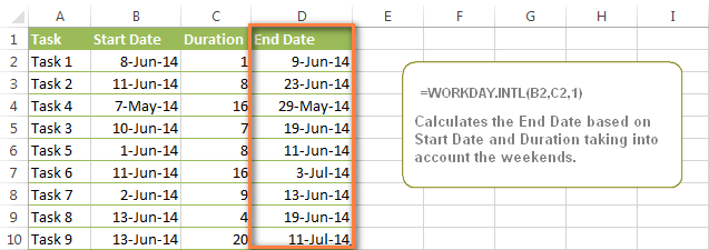
In the formula, we enter 1 as the 3rd parameter since it indicates Saturday and Sunday as holidays. You can use another value if your weekends are different, say, Fri and Sat. The full list of the weekend values is available here. Optionally, you can also use the 4th parameter [holidays], which is a set of dates (range of cells) that should be excluded from the working day calendar.
And finally, you may want to highlight rows depending on how far away the deadline is. For example, the conditional formatting rules based on the following 2 formulas highlight upcoming and recent end dates, respectively:
=AND($D2-TODAY()>=0,$D2-TODAY()<=7)- highlight all rows where the End Date (column D) is within the next 7 days. This formula is really handy when it comes to tracking upcoming expiration dates or payments.=AND(TODAY()-$D2>=0,TODAY()-$D2<=7)- highlight all rows where the End Date (column D) is within the last 7 days. You can use this formula to track the latest overdue payments and other delays.
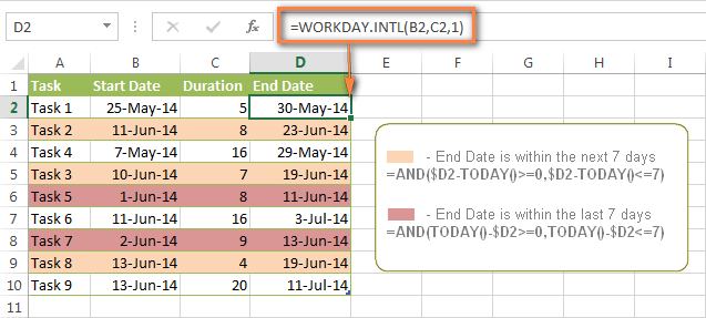
Here are a few more formula examples that can be applied to the table above:
=$D2<TODAY() - highlights all passed dates (i.e. dates less than the current date). Can be used to format expired subscriptions, overdue payments etc.
=$D2>TODAY() - highlights all future dates (i.e. dates greater than the current date). You can use it to highlight upcoming events.
Of course, there can be infinite variations of the above formulas, depending on your particular task. For instance:
=$D2-TODAY()>=6 - highlights dates that occur in 6 or more days.
=$D2=TODAY()-14 - highlights dates occurring exactly 2 weeks ago.
How to highlight dates within a date range
If you have a long list of dates in your worksheet, you may also want to highlight the cells or rows that fall within a certain date range, i.e. highlight all dates that are between two given dates.
You can fulfil this task using the TODAY() function again. You will just have to construct a little bit more elaborate formulas as demonstrated in the examples below.
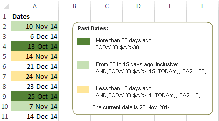
Formulas to highlight past dates
- More than 30 days ago:
=TODAY()-$A2>30 - From 30 to 15 days ago, inclusive:
=AND(TODAY()-$A2>=15, TODAY()-$A2<=30) - Less than 15 days ago:
=AND(TODAY()-$A2>=1, TODAY()-$A2<15)
The current date and any future dates are not colored.
Formulas to highlight future dates
- Will occur in more than 30 days from now:
=$A2-TODAY()>30 - In 30 to 15 days, inclusive:
=AND($A2-TODAY()>=15, $A2-TODAY()<=30) - In less than 15 days:
=AND($A2-TODAY()>=1, $A2-TODAY()<15)
The current date and any past dates are not colored.

How to shade gaps and time intervals
In this last example, we are going to utilize yet another Excel date function - DATEDIF(start_date, end_date, interval). This function calculates the difference between two dates based on the specified interval. It differs from all other functions we've discussed in this tutorial in the way that it lets you ignore months or years and calculate the difference only between days or months, whichever you choose.
Don't see how this could work for you? Think about it in another way… Suppose you have a list of birthdays of your family members and friends. Would you like to know how many days there are until their next birthday? Moreover, how many days exactly are left until your wedding anniversary and other events you wouldn't want to miss? Easily!
The formula you need is this (where A is your Date column):
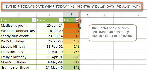
=DATEDIF(TODAY(), DATE((YEAR(TODAY())+1), MONTH($A2), DAY($A2)), "yd")
The "yd" interval type at the end of the formula is used to ignore years and calculate the difference between the days only. For the full list of available interval types, look here.
Tip. If you happen to forget or misplace that complex formula, you can use this simple one instead: =365-DATEDIF($A2,TODAY(),"yd"). It produces exactly the same results, just remember to replace 365 with 366 in leap years : )
And now let's create an Excel conditional formatting rule to shade different gaps in different colors. In this case, it makes more sense to utilize Excel Color Scales rather than create a separate rule for each period.
The screenshot below demonstrates the result in Excel - a gradient 3-color scale with tints from green to red through yellow.
"Days Until Next Birthday" Excel Web App
We have created this Excel Web App to show you the above formula in action. Just enter your events in 1st column and change the corresponding dates in the 2nd column to experiment with the result.
If you are curious to know how to create such interactive Excel spreadsheets, check out this article on how to make web-based Excel spreadsheets.
Hopefully, at least one of the Excel conditional formats for dates discussed in this article has proven useful to you. If you are looking for a solution to some different task, you are most welcome to post a comment. Thank you for reading!
 by
by
1208 comments
I have 3 columns in excel:
- Plan Duration Days (e.g.: 15)
- Start Date (e.g.: 1-June-2015)
- Available days / week (e.g.: 3)
Expected Completion Date: 1-July-2015
Can I calculate expected completion date from the excel formula?
Hi,
I'm running a transport system, and I need to track where my trucks are at a particular point in time.
I have an ETA (Expected Time of Arrival) for all the drivers according to their destinations.
Now, I need a conditional formatting rule to show (in colors) how long a driver spends on his journey at these three points using the commencement date.1. Workshop 2. In-transit 3. Customer Outlet
Eg. Customer A outlet takes 5 days to arrive. The driver spends two days in the workshop (I need this column to show green), he spends another 3 days in-transit (this should still show green), and he arrives at the customer's location on the sixth day (this will show amber) as he is behind target.
Regards,
Reagan
Hello-
I have read through all of the questions on this page and didn’t see this specific question asked. I would greatly appreciate your assistance!
I have an excel worksheet- starting in column and row D6 (start date), E6 (End date), and F6 (Frequency). Across the rows at the top we have weeks starting in column and row G4, H4, I4, etc = (July 13, July 20, July 27), etc.
My first conditional format- to color in the weeks where a communication was sent, worked. That formula was: =AND(G$4$D6) and it applied to: =$G$6:$AM$38
This worked well for the rows with the frequency of daily or weekly. Where we are struggling with is conditionally formatting rows to fill cells with monthly repetition.
Currently, the formula I have: =AND(G$4$D7) is for a specific row i.e. applies to: =$G$7:$AN$7 and this highlights the specific cell that corresponds to the week of the first date that the communication was sent out.
My first question:
1) How do I create a specific conditional formatting rule using the =AND(G$4$D7) formula that fills in a cell every 30 days or 1 month and also corresponds to the correct week, leaves the remainder of the cells blank for that row, and that also ends when the end date in column E says? Will I have to have 2 separate formulas for each row with a monthly frequency? One for filling in the cells, the other for shading the remainder blank? Also, I should be able to specify in one rule that the formula applies to row 7, 10, 15, 22 for example in the “Applies to” section without having to make a new rule for each row, correct?
2) What is the order in the rules manager that these rules should be placed? Should the original formula for all cells be placed at the top or bottom?
Thank you in advance for the help.
Ok think I have a mission imposable here, I need to do an “if, than conditional formatting”. So column “A” is the item “B” is the Due date and “C” is the delivery date. So I need the date in Column “B” to be Green if “C” is blank and “B” is greater than 120 days out, Yellow if “C” is blank and “B” is 60-120 days out and Red if “C” is blank and “B” is less than 60 days out. Is this even possible?
Hi Chris,
Of course, it's possible. If my understanding is correct, "greater than 120 days out" means more than 120 days from the current date. If so, you can create 3 rules based on the following formulas (assuming that row 2 is your top-most row with data):
Green: =AND($C2="", $B2-TODAY()>120)
Yellow: =AND($C2="", $B2-TODAY()>=60, $B2-TODAY()<=120)
Red: =AND($C2="", $B2-TODAY()<60)
I want cells to turn red if date is within 30 days of maturity date, turn green if within 15 days and turn yellow if within 3 days.
For Ex if Maturity date is 07-Apr-2016, I need that cell to be red if date(current) is 07-Mar-2016 and so on.
Please advise formulae to be used for above.
Hi Nick,
Assuming that the Maturity date is in cell A1, you can create 3 rules based on the following formulas:
Red: =AND($A$1-TODAY()<=30, $A$1-TODAY()>15)
Green: =AND($A$1-TODAY()<=15, $A$1-TODAY()>3)
Yellow: =AND($A$1-TODAY()<=3, $A$1-TODAY()>0)
Hi,
I'm trying to build a gantt chart and I'm stuck with conditional formatting. I'm trying to fill up the total number of working days excluding the weekend.
Basically I have,
[dur][start][end=(start)+(dur)-1][completion-%]
My current formula,
This is to highlight the date
=AND(AND(J$4>=$F8,J$4<=$G8),$A8"")
This is to highlight the completion percentage
=AND($A8"",$H8>0,J$4>=$F8,J$4<=($F8+$H8*($G8-$F8)))
Is there a way to use skip the weekend?
Hi,
I have a large spreadsheet with a column containing dates, and need to have a column next to this one which names which year the date falls into.
Eg, if a date is between 01/08/12 and 31/07/13 the 2nd column needs to say "year 1", 01/08/13 - 31/07/14 is "year 2" and so on.
I'm sure this should be fairly simple I just cant work it out!!
Hi Roy,
You don't need conditional formatting in this case. Use a nested IF function similar to this:
=IF(AND(A1>=DATEVALUE("1-Aug-2012"), A1<=DATEVALUE("31-Jul-2013")), "year1", IF(A1<=DATEVALUE("31-Jul-2014"), "year2", ""))
Hi Svetlana,
That's brilliant, I suspected I was doing something fundamentally wrong!
Thanks for your help!
Roy
Hi,
I'm creating a table for Targeted Dates and Targeted Times, based on Initial Dates and Initial Start Time. How do I format a cell, if using 24hr clock, if a time (midnight) falls into the next day? I need the cell to calculate to the following day, based on the time, but it should also remain the current date if time falls within the current time frame. Hope this makes sense.
Hi,
I'm creating a resource plan in which I would like to highlight that a resource is available for project work only 3 days a week.
E.g.:
Mr. A works every Thursday on A task (full year)
Mr. A works every Friday on B task (full year)
Mr. A is available for a project from Monday - Wednesday for project/sprint work
I have hard coded formatting for initial 2 logic but not able to apply conditional formatting on 3 days a week. Based upon inputted dates, the formatting is coloring the whole duration however I don't want to apply formatting on Thursdays and Fridays.
Hi -
I am trying to create a visit schedule. I have formatted all of the cells to be in the date format. The initial cell is blank; however, when I insert formulas below to calculate other visit dates that are based on the initial cell a random date will populate. I would like all cells to remain blank until the initial cell is populated with a start date of my choosing. Please advise.
Study Visit Visit Date
Day 1
Day 15 15-Jan-00
Day 30 30-Jan-00
Day 45 14-Feb-00
and that is using todays date as the expire date.
Hi Stacey,
Select the cells in column C that you want to color, begining in C3, and create a rule with the formula =$C3<=TODAY()
I am trying to find a formula to have the cell go red when it hits expiration date, but keeping all others that aren't expired to remain white. there will be only one date entered in c row 3.
hello i wanna learn how overdue date move another sheet automatic and deleted current sheet
Each time a worksheet is amended (each morning)it calculates labour time for the previous day, I want this labour time to occupy other cells on another worksheet for Monday through to Friday. I can get this to happen but I loose the previous days figures.The formula i have used is below, what should the false statement be to keep the whole weeks data in their respective cells.
=IF(WEEKDAY(TODAY(),2)=5,'Cap Plan Data '!O8)
I am trying to do the following:
Track dates and identify if the date in the cell is
Less than 14 days ago
More than 14 days ago
More than 30 days ago
I have tried all possible combinations I can find, but cannot come up with an exact formula.
Thank you
Hello Leslie,
Try the following formulas where A2 is your first row with data.
Less than 14 days ago: =AND(TODAY()-$A2>0, TODAY()-$A2<14)
From 30 to 14 days ago, inclusive: =AND(TODAY()-$A2>=14, TODAY()-$A2<=30)
More than 30 days ago: =TODAY()-$A2>30
Thank you for this post. I have a starting date for clients and need to call at one month after the start, 3 months, and six months. I would like the column to show a color if the call hasn't been completed and it has hit the 1 month, 3 month, and six month marks. I would also like it to not show a color if the call has been completed. Do you know how I can accomplish this?
Column A would be the start date
Column B would be the 1st month with the option to select completed or not completed
Colmun C would be the 3rd month with the option to select completed or not completed
Column D would be the 6th month with the option to select completed or not completed
:) Thanks a Ton. have bookmarked your site. :)
1 Facebook like from me in return. thanks again.
2 removed ad filtering addons from the site.
Best wishes.
Thank you :)
another question:
how to know if two dates fall in the same month?
thanks again :)
Using the MONTH function :)
For example, =MONTH(A1)=MONTH(B1) will display TRUE if the dates fall in the same month, FALSE otherwise.
Thanks for such a quick reply. btw: what should be the format of the cell in which i want the results. i am also now looking into the link being suggested.
thanks again
It can be any date format that you choose. Formatting is only a visual representation, internally dates are stores as numbers and can be displayed in a variety of ways. For more info about Excel date formats, please see:
https://www.ablebits.com/office-addins-blog/change-date-format-excel/
i meant
11/01/2013
11/02/2013
sorry for the double post..
hi
11/1/2013 0:00 is present in cell C3
11/2/2013 0:00 is present in cell C2
formatting of both is "mm/dd/yyyy h:mm"
how can i find the difference/number of days between these two dates.
Thanks in advance.
eagerly waiting.
Hi!
You can simply subtract one date from the other: =C2-C3
Or, you can use the DATEDIF function as demonstrated in How to calculate days between two dates.
I am trying to figure a formula for when how long it is taking cars to go through detail process from when they arrive. What I need is something that would turn the row
Green for today plus 5 day
yellow for 6-10
red for 11+
I have tried several and cannot get it to change the right color.
Please and Thank you
Hi Megan,
Supposing that your dates are in column A beginning in row 2, you can use the following formulas:
Green: =AND($A2-TODAY()>=0, $A2-TODAY()<=5)
Yellow: =AND($A2-TODAY()>=6, $A2-TODAY()<=10)
Red: =$A2-TODAY()>=11
You may have answered this already, and I did not understand it. I am looking to format a spreadsheet so that when a date is entered in column B, three days later the cell in Column D highlights in red. In the days between, the cell should be highlighted in a lighter color.
Thanks for your help!
Good day, Svetlana,
I've glanced through your forum to see if I could find a place where you've already answered, but saw one similar still blank. So I'll ask again for both of us!
I have dated certifications that are due every year. However, for inspection, I can't put in the due date and use the common TODAY function that most people use to get 90/60/30 days out from being due. Mine has to incorporate the last completion date counting down to when it is due again next year. I'm looking for a formula that will use today's date, reference the column with last completion dates, and tell me when they are 90-61/60-31/30-1/0-past due. If you could help me and suggest which one of the new rule choices to select and enter it into, I would much appreciate it!
Have a Great Evening!
~HLA
Good time of day! :)
Supposing the last completion dates are in column A, you can create rules with the following formulas:
90-61: =AND($A2-TODAY()>60, $A2-TODAY()<=90)
60-31: =AND($A2-TODAY()>30, $A2-TODAY()<=60)
30-1: =AND($A2-TODAY()>0, $A2-TODAY()<=30)
0-past due: =TODAY()-$A2>=0
Svetlana, hello!
I must thank you, Lady. I very much appreciate your expertise, and wish you a wonderful day!
Hi!
I've got to create a spreadsheet and I'm totally overwhelmed!
I need to have future dates assigned to particular cells and I need to have those cells become highlighted a month before this date. Does that make sense and what would be the best way to do that?
Best,
M
Hi Margarita,
Supposing that your future dates are in column A and begin in cell A2, you can use the following formula:
=AND($A2-TODAY()>0, $A2-TODAY()<=30)
Hello,
I am having issues with a date formula. I have a spreadsheet with an end date of 5/1/2015 in C3. I then have dates in column B which need to be conditionally formatted to turn green, yellow, or red depending on how far they are from 5/1/15. For example, my date of 4/30/15 needs to be green (one business day prior), 4/29/15 needs to be yellow (2-3 business days prior), and 4/27/15 or before (more than 3 business days prior to date in C3) needs to be red. I hope this makes sense. Please let me know if you need more information - I have tried everything I can think of!
Hi,
One of the best and most clear examples i have come across. LOVE IT! straight forward and clear!
I do however struggle with the following.
*Start Date*
Confitional format for 3 - 6 months from start
Confitional format for 6 - 9 months from start
Confitional format for 9 - 12 months from start
Confitional format for 12 - 18 months from start
Confitional format for 18 - 24 months from start
Confitional format for 24 months from start
I have looked at your method for days but im unsure if this works the same for months.
would it make sense to calculate days separately to then use that (hidden colomn) to do conditional formatting??
Any advise appreciated.
Keep up the great work
Hi Alex,
Thank you so much for your kind words.
As for your task, you can use the Excel DATEDIF function to calculate the difference between the start date and other dates in months.
For example, a rule with the following formula will format dates that are 3 - 6 whole months after the start date, inclusive:
=AND(DATEDIF($A$1, $B2, "m")>=3, DATEDIF($A$1, $B2, "m")<=6)
Where A1 is the start date and B2 is the top-most cell in the column of dates you want to format.
Thank you soo much for the fast response and a solution.
been wrecking my brain for 3 days with this.
will respond back with the outcome.
I am trying to set up a task tracker with forecast and actual dates. A date that is forecasted and is past due should turn red. a date that is forecasted and only 7 days away should turn yellow and any actual dates should remain standard font. Please help!
Hi,
I can't get the different colours to work, but highlighting in one colour is still a massive help. Thank you so much!
Hi, Could you please help me!!
I am trying to make a spreadsheet to show the first contact with a company (in the C cells), the F cells show the date 42 days which is the first follow up appointment due (which is where I need the colour coding highlighting system to increase awareness of the date) and the third column (G3, etc) will be the date the follow up appointment is completed (which will mean I no longer need the highlighting assistance).
I currently have cells F3-F200 with the formula =IF(C3="","",C3+42) etc, to calculate the date 42 days on from the date in the C cells. I would like to put a conditional formatting formula on the F cells which tells me if the date is approaching. I would like it to be highlighted red if due within a week of the current date (and stay red if it goes past the date) and orange if it is due within 2 weeks of the current date. However, I would also like the highlighting to go away once the new date has been put in the column next to it (which will be G3-G200 - these cells have no formulas or data in them until).
Please help, I'm so stuck!!
Thanks :)
Hi Nicole,
Try the following rormulas:
Red: =AND($G3="", TODAY()-$F3<=7)
Orange: =AND($G3="", AND(TODAY()-$F3<=14, TODAY()-$F3>7))
Good afternoon,
I have a checklist spreadsheet that i am working on and need some assistance with conditional formatting. I have one column which has dates in it. I want to use an icon set for the following:
When the date is today or any future date I want the green icon.
When the date is within 14 days of today's date I want the icon to be orange - this needs to change and each day passes (a date 3 weeks from today would be green but as soon as it reaches the 14 days to go mark, I want it to turn to orange.
Any date that is before today's date would be red.
I can get the red and green to work but not the orange. Please help.
Thanks
Marc
Hi Marc,
The green and red icons are easy, please see the settings below. As for the orange one, sorry I cannot figure out a proper formula because relative cell references are not allowed for icon sets.
Hi, im stuck, just learning excel. How do you create a formula that shows how many days left til the end of the month. Am assuming I use a NOW function, just not sure how to do it.
Thankyou in advance. =)
Hi Karen,
You can use either formula:
=EOMONTH(TODAY(), 0)-TODAY()
or
=DATEDIF(TODAY(), EOMONTH(TODAY(), 0), "d")
To display the number of days, a cell with the formula should be in the General format.
You can find more about calculating dates in Excel in our Excel Date tutorial. For example, the following article explains the details of the EOMONTH function that returns the last day of the month:
https://www.ablebits.com/office-addins-blog/excel-month-eomonth-functions/#get-month-last-day
Hi
How to highlight all dates rows above a specific date.
e.g all rows above 1 January, 2019.
thanks
Hello Svetlana,
Can you please advise on my last question to you in post 116? Any help/suggestions would be greatly appreciated. And I can explain further if needs be.
Thanks in advance,
Leon
Hi Leon,
I am sorry I have very little experience with Google sheets. In Microsoft Excel, you could probably do this by using the VLOOKUP function (https://www.ablebits.com/office-addins-blog/excel-vlookup-tutorial/)
Though, I cannot state anything with confidence without seeing your data structure. If you could post this question on our forum and attach a sample Excel workbook for better understanding, our support team will do their best to help.
HI,
How can we highlight the data upto current month in conditional formats ..
Thank you in advance.
Hi Sai,
Assuming that your dates are in column A and row 2 is the first row with data, you can create a rule with the following formula:
=$A2<DATE(YEAR(TODAY()),MONTH(TODAY()),1)
Hello Svetlana,
Really hope you can help me.
I manage a spreadsheet (on Google Sheets), that lists booked on adverts that have specific copy deadlines for each ad. Each ad copy deadline is dependant on the section of the paper in which it appears. So, for example, for an ad appearing in Sport/Main News section deadline is always the day before. For an ad appearing in Weekend magazine, copy deadline is 10 days before, Review section, 4 days before and so on.I have separate columns for Section name, Publication Date, Copy deadline.
Is there a method or formula I could use that could automatically tell me the copy deadline of the ad, based on the section in which it appears and publication date? So if I enter the section name, and the publication date, the copy deadline will appear with the correct deadline date.
Thanks in advance.
i have a spreadsheet which i import data from a .csv file daily and run a report to show missed telephone calls. I want to highlight those times when the office is open but can't seem to get conditional formating to just look at the times. The format the date/time info is in is 15/05/2015 12:33, i just want to highlight the time if between certain times and not the date as this changes daily with each import. can onlt get the formatting if i include the date and time. Any suggestons? Thanks
Hello Mark,
Please select the Timestamp column and create a rule using this formula:
=AND( TIMEVALUE("10:10")<=(D2-INT(D2)),(D2-INT(D2))<=TIMEVALUE("17:00"))
Where D2 is the first cell in your selection
"10:10" – "17:00" is the time range that you want to highlight.
I am looking for a function that will tell me when my invoice dated 1/1/2015
is over 30, 60 or 90 days..
Hi Becky,
Assuming that your invoice date is in cell A2, you can use the following formulas:
Over 30 days: =TODAY()-$A2>30
Over 60 days: =TODAY()-$A2>60
Over 90 days: =TODAY()-$A2>90
Hi Svetlana Cheusheva ,
Could you pleas tell me how to highlight a cell (Say A1) if the cell value (Say B1) is of the last month date.
Thanks in advance.
Hi Abhishek,
Here's the formula:
=MONTH($B1)=MONTH(TODAY())-1
I have an excel sheet where I am highlighting completion dates with respect to current date. The formula am using is =AND($P6-TODAY()>=0,$P6-TODAY()<=7). Here P6 stores the cut-off date. However am also trying to match it with another criteria in column L6 which stores whether the job has been completed or is in-progress. All am looking to do here is if job completionYes and the completion date<=7 days from current date then such completion dates should be marked in RED.Pls help, thank you
I have tryed some of the above examples with no luck. I have a spread sheet with names in colum A and dates in colum C if the dates are more than 3 months old I want to highlight the names orange, and if the dates are 6 months or greater I want the names to be red. any help?
Thanks
Hi Chris,
Select the cells in column A you want to highlight (not including the column headers) and create the following rules:
Orange: =AND(TODAY()-$C2>90, TODAY()-$C2<180)
Red: =TODAY()-$C2>=180
Assuming that row 2 is your first row with data.
Please note, the formula operate on days, not months, because the number of days differ from month to month.
Hi Svetlana
Please can you help me, I make use of a spread sheet to monitor and track all certificates expiry’s for all of my employees, I would like the cells to automatically change colour if the date has expired + going to expire in 0-30 days, 0-60 days, 0-90 days.
Thanks so much.
Hi Etienne,
Assuming that your dates are in column A, you can use the following formulas:
Expired:=$A2<TODAY()
Expire in 0-30 days: =AND($A2-TODAY()>=0, $A2-TODAY()<=30)
Expire in 31-60 days: =AND($A2-TODAY()>30, $A2-TODAY()<=60)
Expire in 61-90 days: =AND($A2-TODAY()>60, $A2-TODAY()<=90)
we can calculate the no of day like =datedif(c11,d1"d")
now how we can calculated the number of months between 31/10/2012 to 31/03/2015
I have a large file that is used to track leased property. Out Leases run for 10 years with 2 10 year extensions. How can I highlight an entire row in red when the lease inception date is coming up on renewal? That is: inception date 1996, renewal is 2016. I don't need exact dates, years will work fine.
I have looked thru your article, but didn't see how to handle a ten year gap.
Thank you for your article and help.
Joe
I need a rule for column C that highlights the cell if the date is 6 months or more in the past.
Hi Dan,
In this case, you can operate on days, not months, because months have a different number on days.
For example the following formula highlights dates that are 180 days or more in the past:
=TODAY()-$C2>180
Hi,
I have an excel spreadsheet (2010) that I would like the date entered in a set cell to turn yellow within that cell three months before it's anniversary. Then to turn red on it's anniversary date.
Any help much apprecaited.
Thanks
Hi,
I need to check the Datetimestamp in an cell and condition format it with different color.
Eg:
Cell content will be in the below format ("22-MAR-15 23:15") ("DD-MON-RR hh:mm") format
Scenario:
o Green when process is complete by 3:00 CST/4:00 EST
o Yellow when process is complete after 3:00 CST/4:00 EST and before 4:00 CST/5:00 EST
o Red when process is complete after 4:00 CST/5:00 EST
Applies to the current date.
Can someone please help me on this.
Thanks
Hi Svetlana! Posted a comment previously, here are some changes to the question.
Here are some details of the matrix:
F1: Data Received Date
G1: Duration (Days excluding weekends)
H1:End Date (Days excluding weekends)
I1: Data Reviewed Date
G2: 3
H2: 4
What needs to be done is that: The date on F ( Data received) has to be added to the end date to calculate the deadline.
If the deadline is met and completed, the cells at I(Data Reveiwed Date) should turn green.
However, if the deadline is not met but it is still completed, it should turn yellow.
I am unable to get the appropriate formulas. Do help, thank you so much.
Hello, I have a .CSV file, which opens in Excel. In the spread sheet, column A is Subject and Column B is the Date. I want to use different colours in Column A (Subject), based on the value in column B (Date). What should be the formula. Thanks for understanding and cooperation.
Hi Svetlana,
I am creating a to do list to coordinate with the various items I have to complete by certain dates but I don't have the knowlege to make up the formula to return what I need.
For instance;
I will get a date or confirmation for a document to be filed and place that Date in A2.
What I need to be able to do is have some cells return a value of 'due within the 15 days prior' and some cells to return a value of 'due within the 15 days after'
I have a spread sheet with employee names and available certifications. The cells are marked with a check if the employee has the certificate. some certificates have expiration dates. I need a formula, for conditionally formatting the individual cells, that changes the color of the check mark when the certificate has expired.