From this article, you'll learn how to unhide columns in Excel 2016 - 2007. It will teach you to show all hidden columns or just the ones you select, how to unhide first column, and more.
The possibility to hide columns in Excel is really helpful. It's possible to conceal some columns by using the Hide feature or by setting the column width to zero. If you happen to work with Excel files where some columns are hidden, you may want to know how to unhide columns in Excel to view all data.
In this post I'll share how to show hidden columns using the standard Excel Unhide option, a macro, the Go To Special functionality and Document Inspector.
How to unhide all columns in Excel
Whether you have one or several hidden columns in your table, you can easily display them all at once using the Excel Unhide option.
- Click on a small triangle in the upper-left corner of your table to select the entire worksheet.
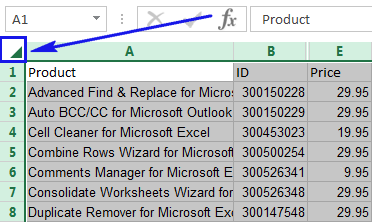
Tip. You can also press the keyboard shortcut Ctrl+A several times until the entire list is highlighted.
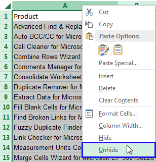
- Now just right-click the selection and pick the Unhide option from the context menu.
Unhide all columns in Excel automatically with VBA macro
You'll find the macro below really helpful if you often get worksheets with hidden columns and don't want to waste your time on searching and showing them. Just add the macro and forget the unhide routine.
If you don't know VBA too well, feel free to explore its possibilities by reading our article How to insert and run macros.
How to show hidden columns that you select
If you have an Excel table where multiple columns are hidden and want to show only some of them, follow the steps below.
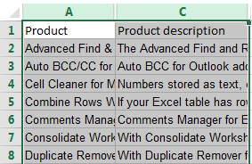
- Select the columns to the left and right of the column you want to unhide. For example, to show hidden column B, select columns A and C.
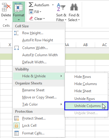
- Go to the Home tab > Cells group, and click Format > Hide & Unhide > Unhide columns.
Or you can right-click the selection and choose Unhide from the context menu, or just press the Unhide columns shortcut: Ctrl + Shift + 0
How to unhide first column in Excel
Unhiding columns in Excel may seem easy until you have several hidden columns but need to display only the left-most one. Pick one of the tricks below to unhide only the first column in your table.
How to unhide column A using the Go To option
Though there is nothing before column A to select, we could select cell A1 to unhide the first column. Here's how:
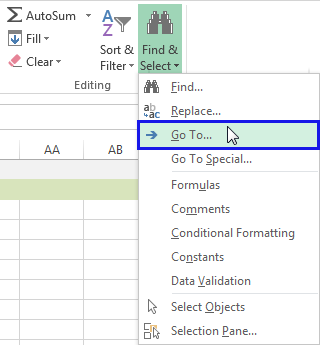
- Press F5 or navigate to Home > Find & Select > Go To…
- You'll see the Go To dialog box. Enter A1 in the Reference: field and click OK.
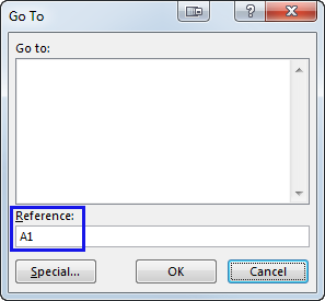
- Although you cannot see it, cell A1 is now selected.
- You go to the Home > Cells group, and click Format > Hide & Unhide > Unhide Columns.

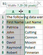
How to unhide the first column by expanding it
- Click on the header for column B to select it.
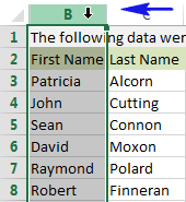
- Move the mouse cursor to the left until you see the double-sided arrow.
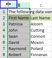
- Now just drag the mouse pointer to the right to expand the hidden column A.
How to unhide column A by selecting it
- Click on the header for column B to select it.

- Drag your mouse pointer to the left until you see the border change its color. It means column A is selected though you don't see it.
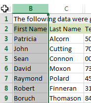
- Release the mouse cursor and go to Home > Format > Hide & Unhide > Unhide Columns.

That's it! This will show column A and leave the other columns hidden.
Show all hidden columns in Excel via Go To Special
It can be rather difficult to find all hidden columns in a worksheet. Of course, you can review the column letters. However, it's not an option if your worksheet contains numerous, like more than 20, hidden columns. Still there is one trick to help you locate hidden columns in Excel.
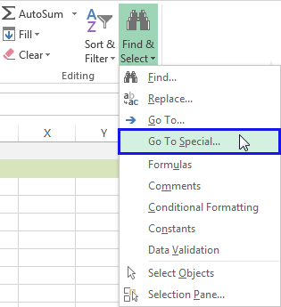
- Open your workbook and navigate to the Home tab.
- Click on the Find & Select icon and pick the Go to Special… option from the menu list.
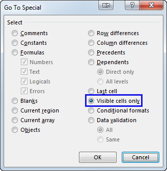
- On the Go To Special dialog box, select the Visible cells only radio button and click OK.
You will see the entire visible part of the table highlighted and the column borders adjacent to the hidden columns borders will become whitish.
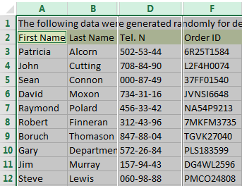
Tip. You can do the same using this short path: F5>Special > Visible cells only. The shortcut funs can just press the Alt + ; (semicolon) hotkey.
Check how many hidden columns there are in a workbook
If you want to check the entire workbook for hidden columns before searching for their location, the Go To Special functionality may not be the best option. You should employ Document Inspector in this case.
- Go to File and click on the Check for issue icon. Select the Inspect Document option. This option examines your file for hidden properties and personal details.
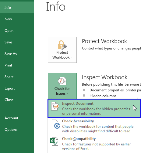
- You may see the notification to save the latest changes before using Document Inspector in order to make sure you keep the important data.

Just click on the Yes or No buttons.
- This will open the Document Inspector window with all the available properties. Make sure the Hidden Rows and Columns option is checked.
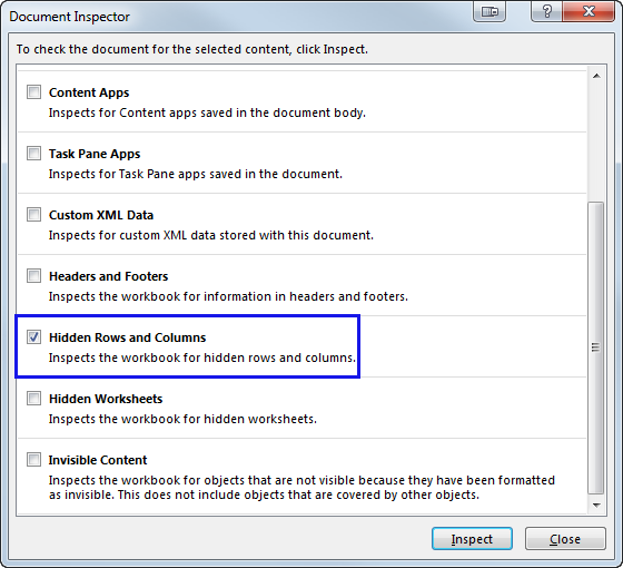
- Press the Inspect button and the tool will start looking for hidden rows and columns.
- As soon as the search is over, you'll see the inspection results.

This window also lets you delete hidden data if you don't trust them. Simply click Remove All.
This feature can appear helpful if you need to know if there are any hidden columns in Excel at all before you navigate to them.
Disable unhiding columns in Excel
Say, you hide some columns with important data like formulas or confidential information. Before you share the table with your colleagues you need to make sure no one will unhide the columns.
- Click on the small Select all icon on the intersection of row numbers and column letters to select the entire table.
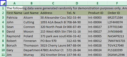
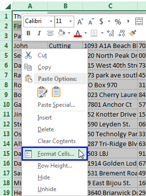
- Right-click on the highlighted list and pick the Format Cells… option from the menu.
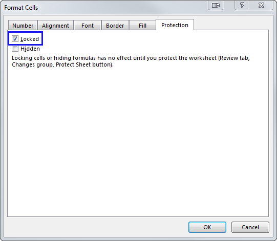
- On the Format Cells window go to the Protection tab and unselect the Locked checkbox.
- Click OK to save the changes.
- Now select the column or columns you want to protect from being unhidden.
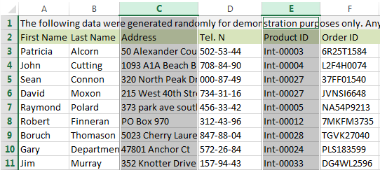
Tip. You can select several columns by keeping the Ctrl button pressed.
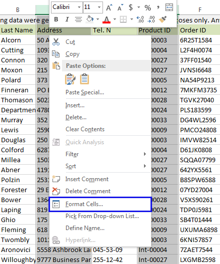
- Click on one of the highlighted columns and select the Format Cells… option again.
- When you see the Format Cells window, navigate to the Protection tab and tick the Locked checkbox.

- Click OK to save the changes.
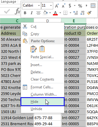
- Hide the columns: select them, right-click and pick the Hide option from the pop-up menu.
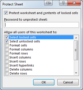
- Now navigate to the Review tab and click on the Protect Sheet icon.

- Make sure the checkboxes Select locked cells and Select unlocked cells are ticked. Then enter and reenter the password.
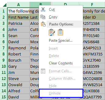
- From now on, anyone who tries to unhide the columns in your Excel table will get the Unhide option disabled.
Note. If you leave any part of the document available for editing a smart person can insert a formula in another column that will refer to your protected hidden column. For example, you hide column A, then another user types =A1 into B1, copies the formula down the column and gets all data from column A in column B.
Now you know how to show hidden columns in your Excel worksheets. Those who prefer to keep their data unseen, can benefit from the possibility to disable the Unhide option. A helpful macro will save your time on unhiding columns every so often.
If any questions left, feel free to comment on the post using the form below. Be happy and excel in Excel!
 by
by
26 comments
To unhide A1, I had to copy/ paste special / Values on a new sheet.... finally got it fixed.
For me column A and B were hidden. I tried all the above but I saw the first column is starting from 'C'.
after seeing the comment section @sandra tan's text gave me that clue. It was frozen. I tired unfreeze pan from View area. It worked. Now am good to go.
thanks a lot
Excellent, Ita really help me.
Thank you so much Charles, yes, my columns were frozen, I thought they were hidden. Now they are visible. Thanks so much for your comment. It's a miracle the network of help we get through internet.
Thanks, unfreeze fixed lot of such unexpected problem in excel.
you just saved me... Thank you!
The Goto Method (Option 1) worked wonders after I had hidden all columns to the right. I (doh) tabbed to another sheet and discovered that the top right cell was XFD1.
The lesson I learned after getting all fired up by a video tutorial to try it out on live data: first hit Ctrl+S!
thanks! the unfreeze rows/column saved me lots of work!
Great blog. Cheers for posting.
I too faced this problem. Unhide did not work as the sheet was freezed after hiding.
So admin to Update this information in the very first step.
Hello!
I could not repeat your situation. Hide - freeze - unhide works. Describe your actions in more detail. Which version of Excel are you using?
Is it possible to disable the unhide function but still able the user to edit the excel document ?
I tried everything to unhide columns -- even what is in this very extensive article -- and no luck. Finally, I tried Unfreezing the top row, and then Unhide worked like magic. So remember, freezing prevents unhiding! Unfreeze, then unhide :-)
Thank you so much!!! I try so hard to find this way.
Also from my side a big thank you for the hint to unfreeze top rows! All the proposals in the article didn't work for me (Excel 2013).
To the authors: would you mind to mention that in the article?
Perfect! Thanks!
Worked and I liked this MAGIC!!!! Finally! Thank you for this hint!
Unfreeze panes!
Worked like MAGIC!!!! Finally! Thank you fort this hint!
Unfreeze panes!
column C to I is hidden, and I saved unknown to me, Pls how do I unhide it? I have tried the unhide option but it's not giving me what I want
That macro didn't work for me in 2013. Is there something that's supposed to come before or after the macro?
Hi! How do I hide a column in excel but dnt gv access to anyone else, meaning if u open my file I dnt want the person to click unhide and read what's on the cell.
I have a column having checkboxes in it in each row. When I hide the column the checkboxes are not hide with the cell data but keep on showing on screen. Is there any way to hide the checkboxes as well?
Hello, Sameen,
Please have a look at this page:
http://stackoverflow.com/questions/18137495/hide-checkboxes-when-hiding-rows
Hope it helps.
i havea pasword protected excelfile of wich i don't have the password, with hidden colums.
is there a wayto make those colums visible.
i tried already to make it a macro with
Sub UnhideAllColumns ()
Cells.EntireColumn.Hidden = False
EndSub
but it didn't work
can anybody help?
it is in excel 2013
Hello, Archie,
I'm really sorry, we cannot help you with this.