How to sort mixed numbers and text, hierarchy numbers in Excel

Sort numbers as text in Excel

When sorting a column of numbers from smallest to largest in Excel, instead of having this:

1, 2, 3, 11, 12, 13, 110, 120, 130

you may sometimes get something like this:

1, 11, 110, 12, 120, 13, 130, 2, 3

That happens when numbers are actually text and they sort as text - like words that are arranged based on their letters, "text-numbers" are sorted based on their digits instead of their values.

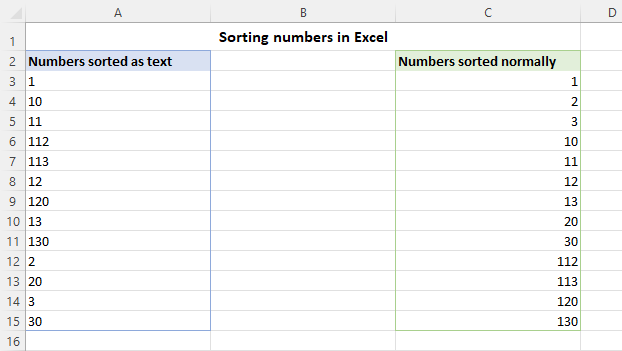
If the target column contains numbers formatted as text, all it takes for the numbers to sort normally is to convert text to number. The result is in column C in the screenshot below.

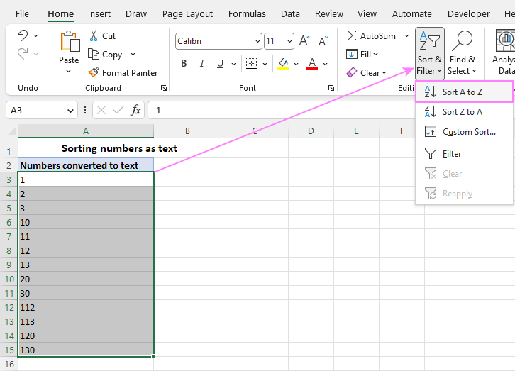
On the contrary, if you wish to sort numbers as text, convert numbers to text first, and then click Home tab > Editing group > Sort & Filter > Sort A - Z.

The result will be like in column A in the previous screenshot.

How to sort mixed numbers and text in Excel

With the built-in Excel Sort feature, alphanumeric strings (combined text and numbers) are always sorted as text, i.e. letter-by-letter, digit-by-digit. To sort a column of numbers containing a letter prefix or suffix as numbers, carry out the steps below. And here's the result we are trying to achieve.

To prevent Excel from handling numbers in alphanumeric strings as text, we're going to extract those numbers in a helper column, and sort by that column. This will let you keep the original data unchanged but rearrange it the way you like.

1. In a column next to the original values, enter a formula that extracts number from string.

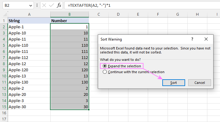
   In this example, we can simply extract all the characters after a hyphen ("-"). In Excel 365, this can be done using the TEXTAFTER function. As with any other Text function, its output is always text, regardless of whether you are retrieving letters or digits, so we multiply the result by 1 to convert a text string to a number.

   =TEXTAFTER(A2, "-")*1

   In older Excel versions, the same result can be achieved using a combination of three different functions that extract text after a specific character. Additionally, the *1 operation is performed to convert the text output to number:

   =RIGHT(A2, LEN(A2) - SEARCH("-", A2)) *1

   Tip. To quickly extract numbers from any position in a cell, you can use the Extract tool included with our Ultimate Suite for Excel.

   
2. Sort the original data by the extracted numbers. With the numbers selected, go to the Home tab > Sort & Filter > Sort Smallest to Largest. In the dialog box that pops up, choose the Expand the selection option and click Sort. For more details, see How to sort and keep rows together.

   Now the strings containing letters and digits are sorted as numbers, and you can remove or hide the helper column if necessary.

Sort strings by text and numbers at a time

In case your source strings have a few different elements, you can extract each element in a separate column, and then sort by multiple columns. As a result, the strings will be arranged like in column D in the screenshot below:

As all the strings in our dataset have the same pattern, the easiest way to split text and numbers into different columns is by using regular expressions. This can be done with the help of the custom function named RegExpExtract. First, you add its code to your Excel as explained in this tutorial. After that, make use of the following formulas.

To extract the first occurrence of text from cell A2, the formula in B2 is:

=RegExpExtract(A2, "[^\d]+", 1)

To extract the first number, the formula in C2 is:

=RegExpExtract(A2, "\d+", 1)*1

To extract the second number, the formula in D2 is:

=RegExpExtract(A2, "\d+", 2)*1

In the 2^nd and 3^rd formulas, we multiply the RegExpExtract output by 1 to turn an extracted substring into a number.

The users of our Ultimate Suite can leverage the Regex Tools to achieve the same result. They will just need to perform one more quick operation to convert the extracted numeric strings (columns C and D) to numbers:

Once the text and numbers are split, sort your dataset by multiple columns:

1. Select all the columns (A2:D16 in our case).
2. On the Data tab, in the Sort & Filter group, click the Sort button.
3. Add as many sort levels as you need and choose the desired sort order.
4. When done, click OK.

In our case, the selected range is first sorted by Text from A to Z, then by Number 1, and then by Number 2 from smallest to largest:

The result is exactly what we were looking for:

How to sort multilevel / hierarchy numbers in Excel

In Microsoft Excel, multilevel numbers such as 1.1, 1.1.1, 1.1.2 are strings, and they sort as text, not numbers:

To sort multilevel strings as numbers, you can use a custom user-defined function that has the following syntax:

Where:

• Range is the range to sort.
• Del is the delimiter used for separating the levels, typically a point (.).
• Max_level is the maximum number of levels in the hierarchy numbers.

And here is the function's code:

What the function does is generate numbers that allow sorting multilevel numeric strings. More precisely, it splits a hierarchy string into individual numbers (parts), processes each part based on the below algorithm, and adds up the results:

part(Index) * (10 ^ ((level - Index) * 2))

For example, for 1.1, the function produces this result:

1*(10^((2-0)*2)) + 1*(10^((2-1)*2)) = 10100

For 1.2, it's:

1*(10^((2-0)*2)) + 2*(10^((2-1)*2)) = 10200

How to sort hierarchy numbers using the custom function:

1. Insert the code of the HierarchyNumber function into a standard code module of your workbook and save it as a macro-enabled workbook (.xlsm). The detailed instructions are here.
2. In a blank cell next to the first hierarchy string, enter a HierarchyNumber formula and press the Enter key.
3. Drag the formula down across as many rows as needed.
4. Sort your dataset based on the column of formulas.

Suppose you have multilevel numeric strings with a maximum of 3 levels in column A. The formula for B2 is:

=HierarchyNumber(A2, ".", 3)

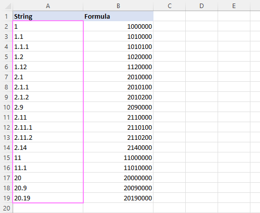
After copying the formula down, you'll get this result:

After that, you sort the whole dataset (A2:B19) by the formula column from smallest to largest:

And get the multi-level numeric strings sorted as numbers:

Sort multilevel numbers prefixed with text

This example discusses a slightly different case where multilevel numbers are prefixed with some text, say "Level 1.1.1". At first sight, the task sounds more complicated, but in fact the solution is simpler :)

First, you extract multilevel numeric substrings into a separate column. For this, you can use the Extract tool included with our Ultimate Suite:

Or you can write a formula to pull all characters after a space:

=RIGHT(A2, LEN(A2) - SEARCH(" ", A2))

And then, do custom sorting. In the Excel Sort dialog box, add two levels - first by the extracted hierarchy number, and then by the original string - and click OK:

The following warning will pop up, where you choose to "Sort numbers and numbers stored as text separately".

As a result, the strings containing multi-level numbers are sorted by numbers:

Available downloads

Sort mixed numbers and text in Excel - examples (.xlsm file)
Ultimate Suite fully-functional trial version (.exe file)