How to sort in Excel by row, column names and in custom order

Sort by several columns

Now I'm going to show you how to sort Excel data by two or more columns. I will do this in Excel 2010 because I have this version installed on my computer. If you use another Excel version, you won't have any problems with following the examples because the sorting features are pretty much the same in Excel 2007 and Excel 2013. You may only notice some differences in color schemes and dialogs' layouts. Okay, let's go ahead...

1. Click the Sort button on the Data tab or Custom Sort on the Home tab to open the Sort dialog.
2. Then click the Add Level button as many times as many columns you want to use for sorting:
   
3. From the "Sort by" and "Then by" dropdown lists, select the columns by which you want to sort your data. For example, you are planning your holiday and have a list of hotels provided by a travel agency. You want to sort them first by Region, then by Board basis and finally by Price, as shown in the screenshot:
   
4. Click OK and you'll get these results:
   • Firstly, the Region column is sorted in the alphabetic order.
   • Secondly, the Board basis column is sorted, so that all-inclusive (AL) hotels are at the top of the list.
   • Finally, the Price column is sorted, from smallest to largest.

   

Sorting data by multiple columns in Excel is pretty easy, isn't it? However, the Sort dialog has plenty more features. Further on in this article I will show you how to sort by row, not column, and how to re-arrange data in your worksheet alphabetically based on column names. Also, you will learn how to sort your Excel data in non-standard ways, when sorting in alphabetical or numerical order does not work.

Sort in Excel by row and by column names

I guess in 90% of cases when you are sorting data in Excel, you sort by values in one or several columns. However, sometimes we have non-trivial data sets and we do need to sort by row (horizontally), i.e. rearrange the order of columns from left to right based on column headers or values in a particular row.

For example, you have a list of photo cameras provided by a local seller or downloaded from the Internet. The list contains different features, specifications and prices like this:

What you need is to sort the photo cameras by some parameters that matter the most for you. As an example, let's sort them by model name first.

1. Select the range of data you want to sort. If you want to re-arrange all the columns, you can simply select any cell within your range. We cannot do this for our data because Column A lists different features and we want it to stick in place. So, our selection starts with cell B1:
   
2. Click the Sort button on the Data tab to open the Sort dialog. Notice the "My data has headers" checkbox in the upper-right part of the dialog, you should uncheck it if your worksheet does not have headers. Since our sheet has headers, we leave the tick and click the Options button.
   
3. In the opening Sort Options dialog under Orientation, choose Sort left to right, and click OK.
   
4. Then select the row by which you want to sort. In our example, we select Row 1 that contains the photo camera names. Make sure you have "Values" selected under Sort on and "A to Z" under Order, then click OK.
   

   The result of your sorting should look similar to this:
   

I know that sorting by column names has very little practical sense in our case and we did it for demonstration purposes only so that you can get a feel of how it works. In a similar way, you can sort the list of cameras by size, or imaging sensor, or sensor type, or any other feature that is most critical for you. For instance, let's sort them by price for a start.

What you do is go through steps 1 - 3 as described above and then, on step 4, instead of Row 2 you select Row 4 that lists retail prices. The result of sorting will look like this:

Please note that it's not just one row that has been sorted. The entire columns were moved so that the data was not distorted. In other words, what you see in the screenshot above is the list of photo cameras sorted from cheapest to most expensive.

Hope now you've gained an insight into how sorting a row works in Excel. But what if we have data that does not sort well alphabetically or numerically?

Sort data in custom order (using a custom list)

If you want to sort your data in some custom order other than alphabetical, you can use the built-in Excel custom lists or create your own. With built-in custom lists, you can sort by days of the week or months of the year. Microsoft Excel provides two types of such custom lists - with abbreviated and full names:

Say, we have a list of weekly household chores and we want to sort them by due day or priority.

1. You start with selecting the data you want to sort and then opening the Sort dialog exactly like we did when sorting by multiple columns or by column names (Data tab > Sort button).
2. In the Sort by box, select the column you want to sort by, in our case it is the Day column since we want to sort our tasks by the days of the week. Then choose Custom List under Order as shown in the screenshot:
   
3. In the Custom Lists dialog box, select the needed list. Since we have the abbreviated day names in the Day columns, we choose the corresponding custom list and click OK.
   

   That's it! Now we have our household tasks sorted by the day of the week:
   

   Note. If you want to change something in your data, please keep in mind that new or modified data won't get sorted automatically. You need to click the Reapply button on the Data tab, in the Sort & Filter group:
   

Well, as you see sorting Excel data by custom list does not present any challenge either. The last thing that is left for us to do is to sort data by our own custom list.

Sort data by your own custom list

As you remember, we have one more column in the table, the Priority column. In order to sort your weekly chores from most important to less important, you proceed as follows.

Perform steps 1 and 2 described above, and when you have the Custom Lists dialog open, select the NEW LIST in the left-hand column under Custom Lists, and type the entries directly into the List entries box on the right. Remember to type your entries exactly in the same order you want them to be sorted, from top to bottom:

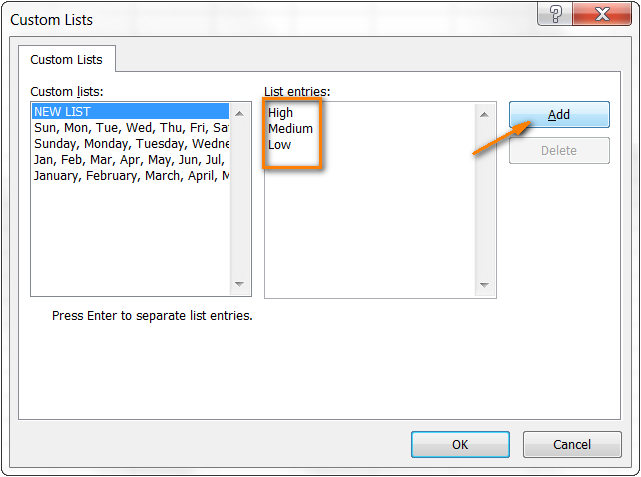
Click Add and you will see that the newly created custom list is added to the existing custom lists, then click OK:

And here come our household tasks, sorted by priority:

When you use custom lists for sorting, you are free to sort by multiple columns and use a different custom list in each case. The process is exactly the same as we have already discussed when sorting by several columns.

And finally, we have our weekly household chores sorted with the utmost logic, first by the day of the week, and then by priority :)