Excel TOROW function to convert range / array to single row

Excel TOROW function

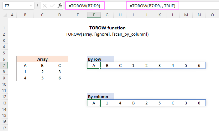
The TOROW function in Excel is used to convert an array or range of cells into one row.

The function takes a total of three arguments, of which only the first one is required.

Where:

Array (required) - an array or range to transform into a single row.

Ignore (optional) - determines whether to ignore blanks or/and errors. Can take one of these values:

• 0 or omitted (default) - keep all values
• 1 - ignore blanks
• 2 - ignore errors
• 3 - ignore blanks and errors

Scan_by_column (optional) - defines how to scan the array:

• FALSE or omitted (default) - scan the array horizontally by row.
• TRUE - scan the array vertically by column.

Basic TOROW formula in Excel

To do a simple range-to-row transformation, use the TOROW formula in its basic form. For this, you need to define only the first argument (array).

For instance, to turn a two-dimensional array consisting of 3 columns and 3 rows into a single row, the formula is:

=TOROW(A3:C6)

You enter the formula into just one cell (A10 in our case), and it automatically spills into as many cell as needed to hold all the results. In Excel terms, the output range surrounded by a thin blue border is called a spill range.

How this formula works:

First, a supplied range of cells is transformed into a two-dimensional array. Please notice the comma-delimited columns and semicolon-separated rows:

{"Apple","Banana","Cherry";1,2,3;4,5,6;7,8,9}

Then, the TOROW function reads the array from left to right and converts it into a one-dimensional horizontal array:

{"Apple","Banana","Cherry",1,2,3,4,5,6,7,8,9}

The result goes to cell A10, from which it spills into the neighboring cell on the right.

Transform range to row ignoring blanks and errors

By default, the TOROW function keeps all the values from the source array, including empty cells and errors. In the output, zero values appear in the place of blank cells, which may be quite confusing.

To exclude blanks, set the ignore argument to 1:

=TOROW(A3:C5, 1)

To ignore errors, set the ignore argument to 2:

=TOROW(A3:C5, 2)

To skip both, blanks and errors, use 3 for the ignore argument:

=TOROW(A3:C5, 3)

The image below shows all three scenarios in action:

Read array horizontally or vertically

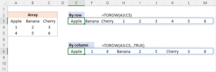
With the default behavior, the TOROW function processes the array horizontally from left to right. To scan the values by column from top to bottom, you set the 3^rd argument (scan_by_column) to TRUE or 1.

For example, to read the source range by row, the formula in E3 is:

=TOROW(A3:C5)

To scan the range by column, the formula in E8 is:

=TOROW(A3:C5, ,TRUE)

In both cases, the resulting arrays are the same size, but the values are arranged in a different order.

Merge multiple ranges into one row

To combine several non-adjacent ranges into a single row, you first stack them horizontally or vertically into a single array with the help of HSTACK or VSTACK, respectively, and then use the TOROW function to convert the combined array into a row.

Depending on your business logic, one of the following formulas will perform the task.

Extract unique values from a range into a row

Beginning with Microsoft Excel 2016, we have a wonderful function, named UNIQUE, that can easily get unique values from a single column or row. However, it cannot handle multi-column arrays. To overcome this limitation, use the UNIQUE and TOROW functions together.

For instance, to extract all the different (distinct) values from the range A2:C7 and place the results in one row, the formula is:

=UNIQUE(TOROW(A2:C7), TRUE)

As TOROW returns a one-dimensional horizontal array, we set the 2nd (by_col) argument of UNIQUE to TRUE to compare the columns against each other.

In case you want the results arranged in alphabetic order, wrap the above formula in the SORT function:

=SORT(UNIQUE(TOROW(A2:C7), TRUE), , ,TRUE )

As with UNIQUE, the by_col argument of SORT is also set to TRUE.

TOROW alternative for Excel 365 - 2010

In Excel versions where the TOROW function is not available, you can transform a range into a single row using a combination of a few different functions that work in older versions. These solutions are more complex, but they do work.

To scan the range horizontally, the generic formula is:

To scan the range vertically, the generic formula is:

For our sample dataset in A3:C5, the formulas take this shape:

To scan the range by row:

=INDEX($A$3:$C$5, QUOTIENT(COLUMN(A1)-1, COLUMNS($A$3:$C$5))+1, MOD(COLUMN(A1)-1, COLUMNS($A$3:$C$5))+1)

This formula is an alternative to the TOROW function with the 3^rd argument set to FALSE or omitted:

=TOROW(A3:C5)

To scan the range by column:

=INDEX($A$3:$C$5, MOD(COLUMN(A1)-1, COLUMNS($A$3:$C$5))+1, QUOTIENT(COLUMN(A1)-1, COLUMNS($A$3:$C$5))+1)

This formula is equivalent to the TOROW function with the 3^rd argument set to TRUE:

=TOROW(A3:C5, ,TRUE)

Please note that unlike the dynamic array TOROW function, these traditional formulas should be entered in each cell where you want the results to appear. In our case, the first formula (by row) goes to E3 and is copied through M3. The second formula (by column) lands in E8 and is dragged through M8.

For the formulas to copy correctly, we lock the range using absolute references ($A$3:$C$5). A named range will also do.

If you've copied the formulas to more cells than needed, a #REF! error will appear in "extra" cells. To fix this, wrap your formula in the IFERROR function like this:

=IFERROR(INDEX($A$3:$C$5, QUOTIENT(COLUMN(A1)-1, COLUMNS($A$3:$C$5))+1, MOD(COLUMN(A1)-1, COLUMNS($A$3:$C$5))+1), "")

How these formulas work

Below is a detailed break-down of the first formula that arranges the values by row:

=INDEX($A$3:$C$5, QUOTIENT(COLUMN(A1)-1, COLUMNS($A$3:$C$5))+1, MOD(COLUMN(A1)-1, COLUMNS($A$3:$C$5))+1)

At the heart of the formula, we use the INDEX function to get the value of a cell based on its relative position in the range.

The row number is calculated by this formula:

QUOTIENT(COLUMN(A1)-1, COLUMNS($A$3:$C$5))+1

The idea is to produce a repeating number sequence such as 1,1,1,2,2,2,3,3,3, … where each number repeats as many times as there are columns in the source range. And here's how we do this:

QUOTIENT returns the integer portion of a division.

For numerator, we use COLUMN(A1)-1, which returns a serial number from 0 in the first cell where the formula is entered to n (total number of values in the range minus 1) in the last cell where the formula in entered. In this example, we have 0 in E2 and 8 in M3.

For denominator, we use COLUMNS($A$3:$C$5)). This returns a constant number equal to the number of columns in your range (3 in our case).

As a result, the QUOTIENT function returns 0 in the first 3 cells (E3:G3), to which we add 1, so the row number is 1.

For the next 3 cells (H3:J3), QUOTIENT returns 1, and +1 gives the row number 2. And so on.

To calculate the column number, you build an appropriate number sequence using the MOD function:

MOD(COLUMN(A1)-1, COLUMNS($A$3:$C$5))+1

As there are 3 columns in our range, the sequence must look like: 1,2,3,1,2,3,…

The MOD function returns the remainder after division.

In E3, MOD(COLUMN(A1)-1, COLUMNS($A$3:$C$5))+1

becomes

MOD(1-1, 3)+1)

and returns 1.

In F3, MOD(COLUMN(B1)-1, COLUMNS($A$3:$C$5))+1

becomes

MOD(2-1, 3)+1)

and returns 2.

Once the row and column numbers are established, INDEX easily fetches the value at the intersection of that row and column.

In E3, INDEX($A$3:$C$5, 1, 1) returns a value from the 1^st row and the 1^st column of the referenced range, i.e. from cell A3.

In F3, INDEX($A$3:$C$5, 1, 2) returns a value from the 1^st row and the 2^nd column, i.e. from cell B3.

And so forth.

The second formula that scans the range by column, works in a similar way. The difference is that we use MOD to calculate the row number and QUOTIENT to figure out the column number.

Practice workbook for download

Excel TOROW function - formula examples (.xlsx file)