In this tutorial, we'll break down the causes of the Excel #NUM error and show you how to fix it.
Are you staring at your computer screen, sipping on your coffee, and wondering why your Excel spreadsheet is suddenly showing a strange error message with the hashtag symbol? It is frustrating, confusing and downright annoying, but fear not! We're here to unravel the mystery of the #NUM error in Excel and help you fix it.
What does #NUM error mean in Excel?
The #NUM error in Excel is a common error message triggered by invalid numeric values, leading to an impossible outcome. This error typically occurs when a function contains incorrect arguments, or when the supplied numbers or dates are not valid numeric values, or when a calculation exceeds the limit of what Excel can handle.
The #NUM error can be resolved in a number of different ways depending on the underlying cause. These can include adjusting input values, changing the formula or calculation, or modifying Excel's calculation settings. A particular solution depends on the specific error and the context of its occurrence.
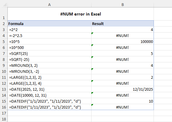
#NUM error in Excel – causes and solutions
Below, we will delve into each possible cause of the #NUM error in more detail and provide you with the necessary steps to resolve it.
Invalid input arguments
Reason: Some Excel functions require specific input arguments. If you provide invalid arguments or incorrect data types, Excel may produce a #NUM error.
Solution: Make sure that all input arguments are valid and of the correct data type. Double-check your formula for syntax errors.
For instance, the DATE function in Excel expects a number between 1 and 9999 for the year argument. If the provided year value is outside this range, the #NUM error will occur.
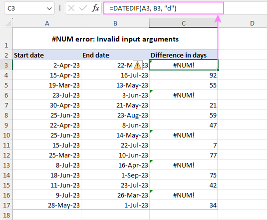
Similarly, the DATEDIF function requires that the end date be always greater than the start date (or both dates are equal). If the opposite, the formula will produce a #NUM error.
For example, this formula will return the difference of 10 days:
=DATEDIF("1/1/2023", "1/11/2023", "d")
And this one will raise the #NUM error:
=DATEDIF("1/11/2023", "1/1/2023", "d")
Too large or too small numbers
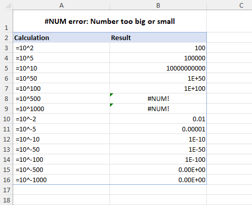
Reason: Microsoft Excel has a limit on the size of numbers that it can calculate. If your formula produces a number that exceeds this limit, a #NUM error occurs.
Solution: If your formula produces a number outside the limit, adjust the input values to ensure that the result falls within the allowable range. Alternatively, you can consider breaking the calculation into smaller parts and using multiple cells to arrive at the final result.
The modern versions of Excel have the following calculation limits:
| Smallest negative number | -2.2251E-308 |
| Smallest positive number | 2.2251E-308 |
| Largest positive number | 9.99999999999999E+307 |
| Largest negative number | -9.99999999999999E+307 |
| Largest allowed positive number via formula | 1.7976931348623158E+308 |
| Largest allowed negative number via formula | -1.7976931348623158E+308 |
If you are not familiar with the scientific notation, I'll briefly explain what it means on an example of the smallest allowed positive number 2.2251E-308. The "E-308" part of the notation means "times 10 to the power of -308", so the number 2.2251 is multiplied by 10 raised to the power of -308 (2.2251x10^-308). This is a very small number that has 307 zeros in the decimal part before the first non-zero digit (which is 2).
As you see, the allowed input values in Excel are between -2.2251E-308 and 9.99999999999999E+307. In formulas, numbers between -1.7976931348623158E+308 and 1.7976931348623158E+308 are allowed. If the result of your formula or any of its arguments is outside the scope, you'll get the #NUM! error.
Please notice that in the current version of Excel 365, only large numbers produce a #NUM error. Small numbers that are outside the limit show up as 0 (General format) or 0.00E+00 (Scientific format). Looks like a new undocumented behavior:
Impossible operations
Reason: When Excel is unable to perform a calculation because it is deemed impossible, it returns the #NUM! error.
Solution: Identify the function or operation that is causing the error and adjust the inputs or modify the formula accordingly.
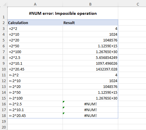
A typical example of an impossible calculation is attempting to find the square root of a negative number using the SQRT function. Since the square root of a negative number cannot be determined, the formula will result in a #NUM error. For example:
=SQRT(25) – returns 5
=SQRT(-25) – returns #NUM!
To fix the error, you can wrap a negative number in the ABS function to get the absolute value of a number:
=SQRT(ABS(-25))
Or
=SQRT(ABS(A2))
Where A2 is the cell containing a negative number.
Another case is the exponentiation of a negative number to a non-integer power. If you try to raise a negative number to a non-integer power, the result will be a complex number. As Excel does not support complex numbers, the formula will produce a #NUM error. In this case, the error indicates that the calculation is impossible to perform within Excel's constraints.
Iteration formula cannot converge
Reason: An iteration formula that cannot find a result causes the #NUM error in Excel.
Solution: Modify the input values to help the formula converge, or adjust the Excel iteration settings, or use a different formula altogether to avoid the error.
Iteration is a feature in Excel that allows formulas to repeatedly recalculate until a certain condition is met. In other words, a formula tries to achieve the result through trial and error. In Excel, there are a number of such functions including IRR, XIRR and RATE. When an iteration formula cannot find a valid result within the given constraints, it returns the #NUM error.
To fix this error, you may need to change the input values or decrease the tolerance level for convergence to ensure that the formula is able to find a valid result.
For example, if your RATE formula results in a #NUM error, you can assist it in finding a solution by providing an initial guess:
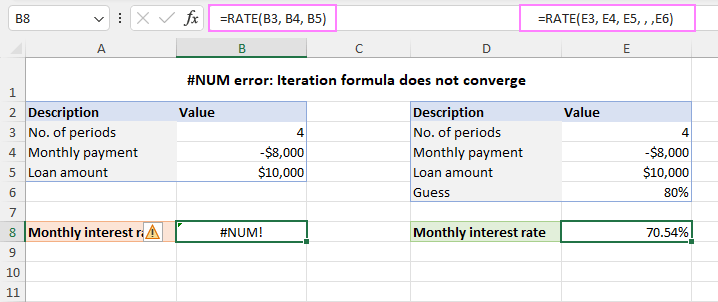
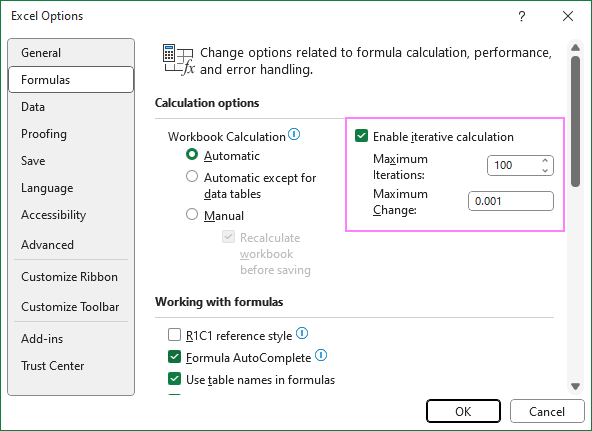
Additionally, you may need to adjust the iteration settings in Excel to help the formula converge. Here are the steps to follow:
- Click on the File menu and select Options.
- On the Formulas tab, under the Calculation options section, check the Enable iterative calculation option.
- In the Maximum Iterations box, enter the number of times you want Excel to perform formula recalculations. A higher number of iterations increases the likelihood of finding a result, but also requires more time to calculate.
- In the Maximum Change box, specify the amount of change between calculation results. A smaller number provides more accurate results but requires more time to calculate.
#NUM error in Excel IRR function
Reason: An IRR formula fails to find a solution due to non-convergence issues or when the cash flows have inconsistent signs.
Solution: Adjust Excel's iteration settings, provide an initial guess, and ensure the cash flows have appropriate signs.
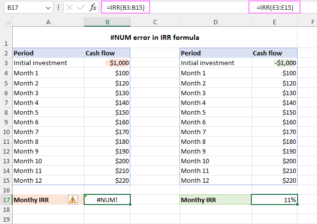
The IRR function in Excel calculates the internal rate of return for a series of cash flows. However, if the cash flows do not result in a valid IRR, the function returns a #NUM! error.
As with any other iteration function, a #NUM error in IRR may occur because of the inability to find an outcome after a certain number of iterations. To resolve the issue, increase the maximum number of iterations or/and provide the initial guess for the return rate (see the previous section for more details).
Another reason why the IRR function may return a #NUM error is due to inconsistent signs in the cash flows. The function assumes that there are both positive and negative cash flows. If there is no change in sign for the cash flows, an IRR formula will result in the #NUM error. To fix this issue, ensure that all outgoing payments, including the initial investment, are entered as negative numbers.
In summary, the #NUM error in Excel is a common issue that can occur for various reasons, including incorrect arguments, unrecognized numbers/dates, impossible operations, and surpassing Excel's calculation limits. Hopefully, this article has helped you understand these reasons and effectively troubleshoot the error.
Practice workbook for download
#NUM error in Excel - examples (.xlsx file)
 by
by
4 comments
how can I avoid "#NUM!" when I use DATEDIF and use a date in the future? I just want it to return blank or "N" or something instead of "#NUM!"
Hi John!
If start date is greater than end date, DATEDIF function returns a #NUM! error. Use IFERROR function to replace error message with a character or word.
I recommend reading this guide: Excel DATEDIF to calculate date difference in days, weeks, months or years.
For example:
=IFERROR(DATEDIF(A1,A2,"d"),"")
I try to follow your recommend formula IFERROR(DATEDIF(A1,A2,"M"),"") but why is invisible the details?
Hi! DATEDIF is one of very few undocumented functions in Excel. Read more here: Excel DATEDIF to calculate date difference in days, weeks, months or years.