An easy way to transform an array or range into a column with the TOCOL function.
The ability to transpose data from columns to rows and in reverse has been in Excel for quite a while. But converting a range of cells into a single column was a tricky task to crack. Now, that's finally changing. Microsoft has introduced a new function, called TOCOL, which can do an array-to-column transformation in a blink. Below is a list of tasks that this new function can easily solve.
Excel TOCOL function
The TOCOL function in Excel converts an array or range of cells into a single column.
The function takes three arguments, but only the first one is required.
Where:
Array (required) - an array or range to transform into a column.
Ignore (optional) - defines whether to ignore blanks or/and errors. Can be one of these values:
- 0 or omitted (default) - keep all values
- 1 - ignore blanks
- 2 - ignore errors
- 3 - ignore blanks and errors
Scan_by_column (optional) - determines whether to scan the array horizontally or vertically:
- FALSE or omitted (default) - scan the array by row from left to right.
- TRUE - scan the array by column from top to bottom.

Tips:
- To convert an array into a single row, use the TOROW function.
- To do the opposite column-to-array transformation, use either the WRAPCOLS function to wrap by column or the WRAPROWS function to wrap by row.
- To transpose an array from horizontal to vertical or vice versa, i.e. change rows to columns, utilize the TRANSPOSE function.
TOCOL availability
TOCOL is a new function, which is supported in Excel for Microsoft 365 (for Windows and Mac) and Excel for the web.
Basic TOCOL formula to transform range into column
The TOCOL formula in its simplest form requires just one argument - array. For example, to place a two-dimensional array consisting of 3 columns and 4 rows into a single column, the formula is:
=TOCOL(A2:C5)
The formula is entered only in one cell (E2 in this example) and spills into the below cells automatically. In terms of Excel, the result is called a spill range.

How this formula works:
Technically, the range A2:C5 is first converted into a two-dimensional array. Please notice the semicolon-separated rows and comma-delimited columns:
{"Apple","Banana","Cherry";1,0,3;4,#N/A,6;7,8,9}
The TOCOL function scans the array from left to right and transforms it into a one-dimensional vertical array:
{"Apple";"Banana";"Cherry";1;0;3;4;#N/A;6;7;8;9}
The result is placed in cell E2, from which it spills into the below cells.
How to use TOCOL function in Excel - formula examples
To gain more understanding of the possibilities of the TOCOL function and what tasks it can cover, let's take a look at some formula examples.
Transform array to column ignoring blanks and errors
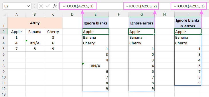
As you may have noticed in the previous example, the default TOCOL formula keeps all the values from the source array, including blank cells and errors.
In the resulting array, empty cells are represented by zeros, which may be quite confusing, especially if the original array has 0 values. The solution is to skip blanks. For this, you set the 2nd argument to 1:
=TOCOL(A2:C5, 1)
To ignore errors, set the 2nd argument to 2:
=TOCOL(A2:C5, 2)
To exclude both, blanks and errors, use 3 for the ignore argument:
=TOCOL(A2:C5, 3)

Scan array horizontally or vertically
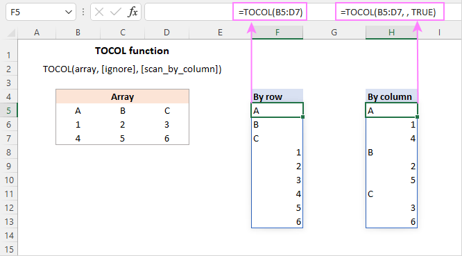
With the default scan_by_column argument (FALSE or omitted), the TOCOL function scans the array horizontally by row. To process values by column, set this argument to TRUE or 1. For example:
=TOCOL(A2:C5, ,TRUE)
Notice that, in both cases, the returned arrays are the same size, but the values are arranged in a different order.

Combine multiple ranges into one column
If you are dealing with several non-contiguous ranges, then you can first combine the ranges vertically into a single array with the help of the VSTACK function, and then use TOCOL to transform the combined array into a column.
Assuming the first range is A2:C4 and the second range is A8:C9, the formula takes this form:
=TOCOL(VSTACK(A2:C4, A8:C9))
This formula demonstrates the default behavior - reads the combined arrays horizontally from left to right as shown in column E in the image below.
To read values vertically from top to bottom, you set the 3rd argument of TOCOL to TRUE:
=TOCOL(VSTACK(A2:C4, A8:C9), ,TRUE)
Please pay attention that, in this case, the formula first returns values from column A of both arrays, then from column B, and so on. The reason is that TOCOL scans a single stacked array, not the original individual ranges.

If your business logic requires stacking the original ranges horizontally rather than vertically, then use the HSTACK function instead of VSTACK.
To append each subsequent array to the right of the previous array and read the combined arrays horizontally, the formula is:
=TOCOL(HSTACK(A2:C4, A8:C10))
To add each subsequent array to the right of the previous array and scan the combined arrays vertically, the formula is:
=TOCOL(HSTACK(A2:C4, A8:C10), ,TRUE)

Extract unique values from a multi-column range
The Excel UNIQUE function can easily find uniques in a single column or row as well as return unique rows, but it cannot extract unique values from a multi-column array. The solution is to use it together with the TOCOL function.
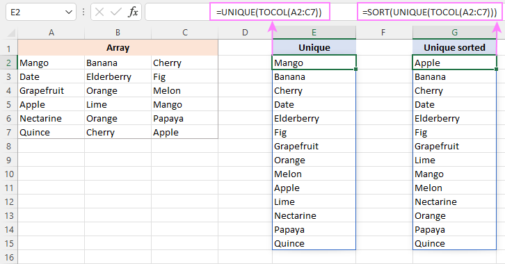
For instance, to extract all the different (distinct) values from the range A2:C7, the formula is:
=UNIQUE(TOCOL(A2:C7))
Additionally, you can wrap the above formula in the SORT function to arrange the returned array in alphabetic order:
=SORT(UNIQUE(TOCOL(A2:C7)))

How to convert range to column in Excel 365 - 2010
In Excel versions where the TOCOL function is not supported, there exist a couple of alternative ways to transform a range of cells into a column. These solutions are quite tricky, but anyway working.
To read the range by row:
To read the range by column:
For our sample dataset, the formulas are as follows:
To scan the range horizontally from left to right:
=INDEX($A$2:$C$5, QUOTIENT(ROW(A1)-1, COLUMNS($A$2:$C$5))+1, MOD(ROW(A1)-1, COLUMNS($A$2:$C$5))+1)
This formula is equivalent to the TOCOL function with the 3rd argument set to FALSE or omitted:
=TOCOL(A2:C5)
To scan the range vertically from top to bottom:
=INDEX($A$2:$C$5, MOD(ROW(A1)-1, ROWS($A$2:$C$5))+1, QUOTIENT(ROW(A1)-1, ROWS($A$2:$C$5))+1)
This formula is comparable to the TOCOL function with the 3rd argument set to TRUE:
=TOCOL(A2:C5, ,TRUE)
Unlike TOCOL, the alternative formulas should be entered in each cell where you want the results to appear. In our case, the formulas go to cells E2 (by row) and G2 (by column), and then are copied down to row 13.
If the formulas are copied to more rows than needed, a #REF! error will appear in "extra" cells. To prevent this from happening, you can nest the formulas in the IFERROR function like this:
=IFERROR(INDEX($A$2:$C$5, QUOTIENT(ROW(A1)-1, COLUMNS($A$2:$C$5))+1, MOD(ROW(A1)-1, COLUMNS($A$2:$C$5))+1), "")
Notice that for the formulas to copy correctly, we lock the range using absolute cell references ($A$2:$C$5). Instead, you can use a named range.

How these formulas work
Below is a detailed break-down of the first formula that arranges cells by row:
=INDEX($A$2:$C$5, QUOTIENT(ROW(A1)-1, COLUMNS($A$2:$C$5))+1, MOD(ROW(A1)-1, COLUMNS($A$2:$C$5))+1)
The idea is to use the INDEX function to return the value of a certain cell based on its relative row and column numbers in the range.
The row number is calculated by this combination:
QUOTIENT(ROW(A1)-1, COLUMNS($A$2:$C$5))+1
QUOTIENT returns the integer portion of a division.
For numerator, you use ROW(A1)-1, which returns a serial number from 0 in E2 (first cell where the formula in entered) to 11 in E13 (the last cell where the formula in entered).
The denominator brough by COLUMNS($A$2:$C$5)) is constant and equals to the number of columns in your range (3 in our case).
Now, if you check the QUOTIENT's result for the first 3 cells (E2:E4), you will see that it's equal to 0 (because the integer part of the division is zero). Adding 1 gives the row number 1.
For the next 3 cells (E5:E5), QUOTIENT returns 1, and the +1 operation delivers the row number 2. And so on.
In other words, this part of the formula creates a repeating number sequence such as 1,1,1,2,2,2,3,3,3,4,4,4,… Each number repeats as many times as there are columns in your range.
To calculate the column number, you build an appropriate number sequence using the MOD function:
MOD(ROW(A1)-1, COLUMNS($A$2:$C$5))+1
As there are 3 columns in our range (A2:C5), the sequence must be 1,2,3,1,2,3,…
The MOD function returns the remainder after division.
In E2, MOD(ROW(A1)-1, COLUMNS($A$2:$C$5))+1)
becomes
MOD(1-1, 3)+1)
and returns 1.
In E3, MOD(ROW(A2)-1, COLUMNS($A$2:$C$5))+1)
becomes
MOD(2-1, 3)+1)
and returns 2.
With the row and column numbers established, INDEX has no problems fetching the required value.
In E2, INDEX($A$2:$C$5, 1, 1) returns the value from the 1st row and the 1st column of the referenced range, i.e. from cell A2.
In E3, INDEX($A$2:$C$5, 1, 2) returns the value from the 1st row and the 2nd column, i.e. from cell B2.
And so forth.
The second formula that scans the range by column, works in a similar way. The difference is that it uses MOD to get the row number and QUOTIENT to get the column number.
TOCOL function not working
If the TOCOL function throws an error, it's most likely to be one of these reasons:
TOCOL is not supported in your Excel
When you get a #NAME? error, the correct spelling of the function's name is the first thing to check. If the name is correct but the error persists, the function is not available in your version of Excel. In this case, consider using a TOCOL alternative.
Array is too large
A #NUM error indicates that the array cannot fit into a column. A typical case is when you refer to entire columns or rows.
There are not enough empty cells
When a #SPILL error occurs, check that the column where the formula is entered has enough empty cells to be filled with the results. If the cells are visually blank, make sure there are no spaces and other non-printing characters in them. For more information, see How to fix the #SPILL error in Excel.
That's how you can use the TOCOL function in Excel 365 and alternative solutions in earlier versions to transform a 2-dimensional array into a single column. I thank you for reading and hope to see you on our blog next week!
Practice workbook
Excel TOCOL function - formula examples (.xlsx file)
 by
by
4 comments
Is there a way to use TOCOL and also get row descriptors as well as column descriptors to transpose?
Jan Feb Mar
Dog 3 2 6
Cat 5 2 1
Fish 4 8 3
converts to
Jan Dog 3
Jan Cat 5
Jan Fish 4
Feb Dog 2
Feb Cat 2
Feb Fish 8
Mar Dog 6
Mar Cat 1
Mar Fish 3
Don't care if month or animal are first or second column?
I have the same query....
THANKYOU
Very very essential tips about learning advance Excel 👌👌