The tutorial explains the syntax of the TRANSPOSE function and shows how to use it correctly to transpose data in Excel.
There's no accounting for tastes. It is also true for work habits. Some Excel users prefer organizing data vertically in columns while others choose horizontal arrangement in rows. In situations when you need to quickly change the orientation of a given range, TRANSPOSE is the function to use.
Excel TRANSPOSE function - syntax
The purpose of the TRANSPOSE function in Excel is to convert rows to columns, i.e. switch the orientation of a given range from horizontal to vertical or vice versa.
The function takes just one argument:
Where array is the range of cells to transpose.
The array is transformed in this way: the first row of the original array becomes the first column of the new array, the second row becomes the second column, and so on.
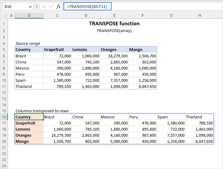
Important note! For the TRANSPOSE function to work in Excel 2019 and lower, you must enter it as an array formula by pressing Ctrl + Shift + Enter. In Excel 2021 and Excel 365 that support arrays natively, it can be entered as a regular formula.
How to use the TRANSPOSE function in Excel
The syntax of TRANSPOSE leaves no room for mistakes when building a formula. A trickier part is to enter it correctly in a worksheet. If you don't have much experience with Excel formulas in general and array formulas in particular, please make sure you follow the below steps closely.
1. Count the number of columns and rows in the original table
For starters, find out how many columns and rows your source table contains. You will need these numbers in the next step.
In this example, we are going to transpose the table that shows the volume of fresh fruit exports by county:
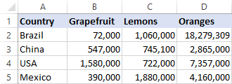
Our source table has 4 columns and 5 rows. Keeping these figures in mind, proceed to the next step.
2. Select the same number of cells, but change the orientation
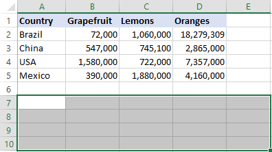
Your new table will contain the same number of cells but will be rotated from the horizontal orientation to vertical or vice versa. So, you select a range of empty cells that occupies the same number of rows as the original table has columns, and the same number of columns as the original table has rows.
In our case, we select a range of 5 columns and 4 rows:
3. Type the TRANSPOSE formula
With a range of blank cells selected, type the Transpose formula:
=TRANSPOSE(A1:D5)
Here are the detailed steps:
First, you type the equality sign, function name and opening parenthesis: =TRANSPOSE(
Then, select the source range using the mouse or type it manually:
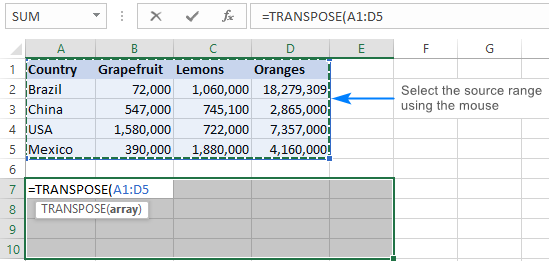
Finally, type the closing parenthesis, but don't hit the Enter key! At this point, your Excel Transpose formula should look similar to this:
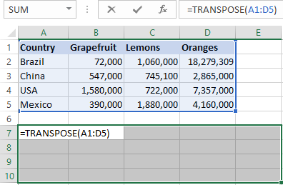
4. Complete the TRANSPOSE formula
Press Ctrl + Shift + Enter to finish your array formula properly. Why do you need this? Because the formula is to be applied to more than one cell, and it is exactly what array formulas are purposed for.
Once you press Ctrl + Shift + Enter, Excel will surround your Transpose formula with {curly braces} that are visible in the formula bar and are a visual indication of an array formula. In no case you should type them manually, that won't work.
The screenshot below shows that our source table was transposed successfully and 4 columns were converted into 4 rows:
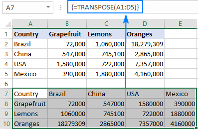
TRANSPOSE formula in Excel 365
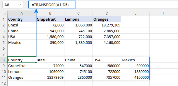
In Dynamic Array Excel (365 and 2021), the TRANSPOSE function is incredibly easy to use! You just enter the formula in the upper-left cell of the destination range and press the Enter key. That's it! No counting rows and columns, no CSE array formulas. It just works.
=TRANSPOSE(A1:D5)
The result is a dynamic spill range that automatically spills into as many rows and columns as needed:
How to transpose data in Excel without zeros for blanks
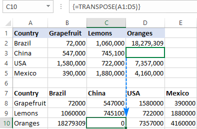
If one or more cells in the original table is empty, those cells will have zero values in the transposed table, as shown in the screenshot below:
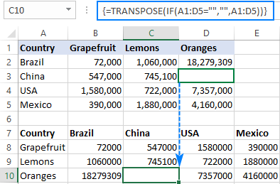
If you wish to return blank cells instead, nest the IF function inside your TRANSPOSE formula to check whether a cell is blank or not. If the cell is blank, IF will return an empty string (""), otherwise supply the value to transpose:
=TRANSPOSE(IF(A1:D5="","",A1:D5))
Enter the formula as explained above (please remember to press Ctrl + Shift + Enter to finish the array formula correctly), and you will have a result similar to this:
Tips and notes on using TRANSPOSE in Excel
As you have just seen, the TRANSPOSE function has a number of quirks that may confuse unexperienced users. The below tips will help you avoid typical mistakes.
1. How to edit a TRANSPOSE formula
As an array function, TRANSPOSE does not allow changing part of the array it returns. To edit a Transpose formula, select the entire range the formula refers to, make the desired change, and press Ctrl + Shift + Enter to save the updated formula.
2. How to delete a TRANSPOSE formula
To remove a Transpose formula from your worksheet, select the whole range referenced in the formula, and press the Delete key.
3. Replace TRANSPOSE formula with values
When you flip a range by using the TRANSPOSE function, the source range and the output range get linked. This means that whenever you change some value in the original table, the corresponding value in the transposed table changes automatically.
If you'd like to break the connection between the two tables, replace the formula with calculated values. For this, select all the values returned by your formula, press Ctrl + C to copy them, right-click, and choose Paste Special > Values from the context menu.
For more information, please see How to convert formulas to values.
That's how you use the TRANSPOSE function to rotate data in Excel. I thank you for reading and hope to see you on our blog next week!
 by
by
11 comments
Hello People,
This blog has been very helpful to me. Many thanks for this. But now I have a weird situation. I have my data blocks in 2 columns. Like the following:
A 24
B 36
C 22.8
A 44
B 31
C 29
What I need is: The first Block's Values (24, 36, 22.8) to form the first row (with A,B,C as column headers), while the second Block's Values (44, 31, 29) to form the second row (under the same column headers: A,B,C)
I have hundreds of blocks of data like this. Performing a manual transpose for each block individually is very time consuming. I was wondering if anyone knows a shortcut to get it done?
Many thanks in advance
Sri
Hello! If your data are written in the range A1:B7, you can try this formula:
=WRAPROWS(VSTACK(A1:A3,TOCOL(B1:B7,1)),3)
For more information, please visit: How to combine ranges / arrays in Excel with VSTACK & HSTACK functions, Convert column / row to range in Excel: WRAPCOLS & WRAPROWS functions and Excel TOCOL function to convert range to single column.
Sir, how do I transpose 16 items into 4 rows and 4 columns?
Such that if I want it spilled over from A1-A4; and then 5th item- instead of A5 it should get into b1.
A 1-4
B 1-4
C 1-4
D 1-4
GET THE ANSWER
A1 A2 A3 A4
FAB10100-S03-S002 WG1419 WG1419 WD2323
WD2323
FAB10100-S03-S002 DFDFDF DFDFDF DFDFDF SSSSSSS
DFDFDF
SSSSSSS
Hi!
If you want help, explain the problem.
Tried it. Doesn't work? Just returns A1, no other records?
Hi Andre,
Remember to press Ctrl + Shift + Enter to complete your formula. Did it work?
thanks a lot, very useful
how would i reference cells that are transposed - meaning in one sheet values are horizontal, and in the other, values are vertical?
Hello!
The reference points to the address of the cell, not the value of the cell. If I understand your question correctly, the link will not change when transposed.
awesome way to rotate data