The tutorial shows how to insert today's date in your worksheets and demonstrates a few other uses of TODAY function in Excel.
You want to put today's date in some cell? Or you wish to highlight the current date in your Excel calendar? Or you'd like to find the date closest to today? All this can be done by using the Excel TODAY function and this tutorial will teach you how.
Excel TODAY function - syntax and basic uses
The TODAY function in Excel does exactly what its name indicates - returns today's date.
The syntax of the TODAY function is as simple as it could possible be - it does not have any arguments at all. Whenever you need to insert today's date in Excel, just enter the following formula in a cell:
=TODAY()
You can format the value returned by TODAY in any built-in or custom date format. For example, this way:

4 things you should know about TODAY in Excel
- TODAY() is a volatile function, which means that it updates itself continuously every time a worksheet is opened or changed.
- If a TODAY formula does not update automatically, most likely automatic recalculation is turned off in your workbook. To turn it on again, go to the Formulas tab > Calculation Options, and select Automatic.
- To enter today's date in Excel as a static unchangeable value, use these keyboard shortcuts.
- If you want to insert current date and time, use the NOW function instead of TODAY.
How to insert today's date in Excel
There are two ways to enter the current date in Excel - a formula and shortcut. Which one to use depends on whether you want a static or dynamic value.
Excel formula for today's date
The value returned by the TODAY function updates automatically, so the below formula is useful if you want the worksheet to always display the current date, regardless of when you open it.
=TODAY()
To clarify what kind of date that is, you can concatenate TODAY() with some explanatory text, for example:
=CONCATENATE("Today is ",TEXT(TODAY(), "mmmm dd, yyyy"))
Because in the internal Excel system dates and times are stored as numbers, concatenating text with the TODAY() formula directly would result in a meaningless string like "Today is 42965". To avoid this, we nest Excel's TODAY function within the TEXT function to display the date in the desired format.

Shortcuts to get today's date in Excel
The inset today's date as an unchangeable timestamp that won't automatically update the next day, use one of the following keyboard shortcuts:
- To inset today's date: Ctrl + ;
- To insert the current time: Ctrl + Shift + ;
- To enter the current date and time: Ctrl + ; then Space and then Ctrl + Shift + ;
How to use TODAY function in Excel - formula examples
As you already know, the main purpose of the Excel TODAY function is to get today's date. Aside from that, you can use TODAY() in combination with other functions to perform more complex calculations based on the current date. Below you will find a few examples of such formulas.
Add or subtract days to/from today's date
To add or subtract a specific number of days to/from the current date, use a simple arithmetic operation of addition or subtraction, respectively.
For example, to add 7 days to todays' date, use this formula:
=TODAY()+7
To subtract 7 days from the current date, go with this one:
=TODAY()-7
To exclude weekends (Saturday and Sunday) from your calculations, nest the TODAY function within WORKDAY that deals with weekdays only:
To add 7 workdays to today's date:
=WORKDAY(TODAY(), 7)
To subtract 7 workdays from today's date:
=WORKDAY(TODAY(), -7)
The following screenshot shows the results:
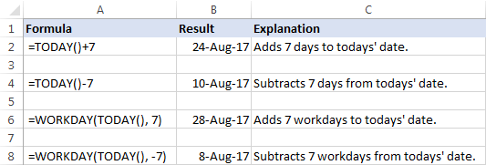
Tip. To display the calculated date correctly, set the formula cell's format to Date.
Get the number of days before or after a certain date
To calculate how many days are left before some data, subtract today's date from the future date you are counting toward:
The date can be supplied directly to a formula in the format that Excel can understand, or by using the DATE function, or as a reference to the cell containing the date.
For example, to find out how many days are left till December 31, 2017, use one of these formulas:
=A2-TODAY()
=DATE(2017,12,31)-TODAY()
="12/31/2017"-TODAY()
All three formulas tell us that at the moment of writing (August 17, 2017), 136 days were left till the end of the year 2017:

To calculate the number of days since a certain date, subtract the past date from today's date:
For example, to find out how many days have passed since January 1, 2017, use one of these formulas:
=TODAY()-A2
=TODAY()-DATE(2017,1,1)
=TODAY()-"1/1/2017"

Tip. If the result is not displayed correct, be sure to apply the General format to the formula cell.
Calculate months since or before a certain date
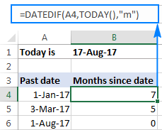
To get the number of months between today and a past date, use the DATEDIF(start_date, end_date, unit) function with the past date in the start_date argument, TODAY() as end_date and "m" unit denoting months:
To get the number of months between today and a future date, swap the start_date and end_date arguments:
With the date of interest in cell A4, use the following formulas to calculate time difference in the number of complete months:
To calculate months since a certain date in the past:
=DATEDIF(A4,TODAY(),"m")
To calculate months before a certain date in the future:
=DATEDIF(TODAY(),A4,"m")
 |
 |
Calculate years since / before a certain date
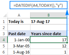
The formulas to calculate years based on today's date are similar to the ones discussed in the above example. The difference is that you use "y" unit to get the number of complete years between today and another data:
To calculate years since a past date:
To calculate years before a future date:
Assuming the past/future date is in cell A4, you should be good with using these formulas:
The number of complete years since date:
=DATEDIF(A4,TODAY(),"y")
The number of complete years before date:
=DATEDIF(TODAY(),A4,"y")
 |
 |
For more information about the DATEDIF function, please see Excel DATEDIF - calculate difference between two dates.
Get age from birthdate
If you know someone's year of birth, you can subtract that year from the current year to find the person's age:
For example, if the person was born in 2000, you use the following formula to get his/her age:
=YEAR( TODAY())-2000
Or, you can enter the year of birth in a separate cell and reference that cell in your formula:

You can learn a few other age calculation formulas in this tutorial: How to get age from date of birth in Excel.
Find the nearest date to today
If you are curious to know which date in a list is closest to today's date, use one of the following array formulas to find it out.
Get a past date closest to today
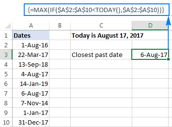
To find a past date nearest to the current date, first "filter out" the dates greater than today, and then use the MAX function to get the largest date among the remaining ones:
With the dates in cells A2 to A10, the formula would go as follows:
=MAX(IF($A$2:$A$10 < TODAY(), $A$2:$A$10))
Get a future date closest to today
To find the nearest future date, identify the dates that are greater than today, and then use the MIN function to get the smallest date among them:
For our sample data set, we'd use this formula:
=MIN(IF($A$2:$A$10 > TODAY(), $A$2:$A$10))
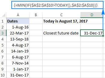
Get any date closest to today
To get the nearest date in a mixed list of past and future dates, use the classic INDEX MATCH formula with a couple of modifications:
Here's how this generic formula works:
- MIN(ABS(range -TODAY())) part. First, you subtract today's date from each date in the range of dates. Then, the ABS function returns the differences as absolute values without regard to their sign. The MIN finds the minimal value, which goes to INDEX MATCH as the lookup value.
- ABS(range -TODAY()) part. You subtract today's date from the range of dates and return an array of absolute values. This array is where INDEX MATCH searches for the lookup value.
In this example, the formula takes the following shape:
=INDEX($A$2:$A$10, MATCH(MIN(ABS($A$2:$A$10 - TODAY())), ABS($A$2:$A$10 - TODAY()), 0))
The screenshot below shows the result:
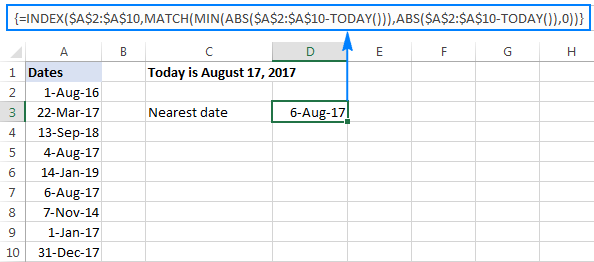
Note. All three formulas to get the nearest date are array formulas, so they should be completed by pressing Ctrl + Shift + Enter.
How to highlight today's date in Excel
When working with a long list of dates or designing your own calendar in Excel, you may want to have the current date highlighted. To have it done, create a conditional formatting rule with this formula:
=B2=TODAY()
Where B2 is the left-top-most cell of the range to which the rule applies.
The result may look something similar to this:
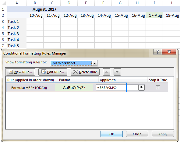
The detailed steps to set up a conditional formatting rule can be found here: How to create a conditional formatting rule based on formula.
To have a closer look at the formulas discussed in this tutorial, you are welcome to download our sample workbook below. Thank you for reading!
Practice workbook for download
Excel TODAY formula - examples (.xlsx file)
More examples of TODAY formula in Excel
For more examples of using the TODAY function in Excel, please check out the following tutorials:
 by
by
169 comments
Question. I am making a spreadsheet for my work and in columb B are dates, some are blank because we have not got that far. Column C is days sence column B. I use =today()-b2 for row 2 and it shows a number lets say 29. Row 3 Column B has no date yet and Column C has the formula =today()-b3 but it displays 45405. Is there a way to hide 45405 or make blank until I put a date into Column B?
Hi! Use the IF function to not do the calculation if the cell is empty. The following tutorial should help: Excel IF statement for blanks and non-blanks cells. For example:
=IF(ISBLANK(B2), "", TODAY()-B2)
Thanks. Worked perfectly.
Hi Team, is there a way to get Day as a value from Today function?
I have tried Text(today(),"dd") but return number as a text.
Thanks for you help.
Hi! To get day of the month, try to use DAY function. For example:
=DAY(TODAY())
Hi :)
I have a sheet that i use Windings 2 - to add a checkmark.
And i want to add todays date/time when i check off the cell with the checkbox. (its; "P") '
How can do that?
Rows i use: L4 to L1000 - and i want date to appear in row: R4 to R1000
Appreciate the help!!
Hi!
If I understand your task correctly, you can insert date when cell value changes using these guidelines: Formula to insert today date & current time as unchangeable time stamp.
Hope this is what you need.
PLS ADVISE FORMULA FOR, (A DATE 30 BY TODAY DATE NEED A AUTO TEXT OF "TRU OR FALS".)
Sorry, I do not fully understand the task.
As it's currently written, it's hard to tell exactly what you're asking.
Is there a way to make =TODAY() update only if the document is changed? We can manually put in a date when we update the sheet, but people tend to forget.
Hi!
TODAY() changes the value when you recalculate formulas and when you open a workbook. The standard features of Excel do not allow you to change TODAY() just when the data changes. This is possible with a VBA macro.
Edit: any time the document is opens, it updates. The article doesn't show a "only if" option
Hello,
Can you help, I’ve a cell A1 with TODAY entered ( formatted to mmm-yyyy). I’m trying to compare A2-A10 containing sequential month and year formatted the same as A1, to produce a transpose sheet if the correct month and year tally up or produce a 0.
I’m using IF(A2= A1, “transpose sheet x”, “0”)
My result alway produce 0 even when A2=A1 eg, Jan-2023=Jan-2023.
Hi! What value is written in A2? I assume that text is written there. If you compare the date to the text, condition A2=A1 will never hold. You can convert the date to text with the TEXT function. For example, TEXT(A1,"mmm-yyyy")
I need a formula, where I mark work as done then in the next column it shows the exact date and that can't be changed.
Hi!
To prevent your date from automatically changing, you can use several methods:
1. Use Shortcuts to insert the current date and time as described above.
2. Use the recommendations from this article in our blog.
3. Replace the date and time returned by the TODAY() function with their values. Copy the date (CTRL + C), then paste only the values using Paste Special or Shortcut CTRL + ALT + V.
i understand what he asked for and i need it also.
i want to add some data to B1 B2 B3 ..etc
whenever i add data to B1, i want excel to autowrite today's date in A1 static.
wheenver i add data to B2 , i want excel to autowrite today's date in A2 as static data.
ctrl+;
is manuel, can we do it autowrite?
Hi! If the recommendations given to you earlier do not suit you, try writing and using VBA code. There are no other standard Excel features.
Is there something for :
If any changes are made in column A-I then column J will update with the current date?
Hi!
Use the TODAY function as described in the article above.
Hi,
How to show on the day of the month, in today() formula.
example: 22 /11/22 ( November 22, 2022), i want to show or extract only the date of month which 22.
thank you
Hi!
If you want to see only the day in the date cell, use the custom date format – "dd".
Is there a way to pull from multiple dates using this? I've been collecting numbers based off of the current date, and have now been asked to pull data by a week instead of daily. I've got TODAY() built into my formula, but want to pull a weeks worth of data without having to change too much of my formula.
Hi!
Without seeing your formula, I can not advise you anything. Explain in detail.
So, I'm pulling data from another workbook and I've been searching by sheet. Is there a way I could even just change it to search the entire workbook rather than just by the sheet. Each time the month changes, I have to change every formula. Due to the large amount of data, I break it the workbook down month by month. Here's my current formula. So currently I'm using Sep2 which represents September 22. At the end of the month, I'll have to go through about 30-40 formulas and update all of them to Oct2.
=COUNTIFS('[COVID-19 Positive 2021.xlsx]Sep2'!$Q:$Q, "Confirmed", '[COVID-19 Positive 2021.xlsx]Sep2'!$N:$N,"<11",'[COVID-19 Positive 2021.xlsx]Sep2'!$U:$U,TODAY())
Hello!
Place the sheet name in a separate cell and insert it into a formula using the INDIRECT function. You can find the examples and detailed instructions here: INDIRECT formula to dynamically refer to another worksheet.
This should solve your task.
The date returned by the TODAY function in Excel updates automatically when your worksheet is recalculated to reflect the current date, which function I should use so that the return date can be fixed.
For example when x=y then return date , and this date should be fixed.
could you please help me in this.
Thanks in advance
Hello!
To prevent your date from automatically changing, you can use several methods:
1. Use the recommendations from this article in our blog.
2. Replace the date and time returned by the TODAY function with their values. Copy the date (CTRL + C), then paste only the values using Paste Special or Shortcut CTRL + ALT + V.
If the total amount is more than rs. 100000 then payment date will be 15 days after inword date
Hi!
I recommend reading this guide: Subtract dates in Excel; add days, weeks, months or years to date.
Hi,
There are two dates available as mentioned below; which are Received date and the Conclude date, from which i can calculate the turnaround time (TAT) as 18 days (Conclude Date - Received date). However i just want to calculate the TAT, if a date available in the Conclude date if not from Todays date. Appreciate your support on creation of a formula.
Received Date Conclude Date TAT
01 Jul 22 19 July 22 18
Hello!
Unfortunately, I don't really understand your issue. You can use any date, not just today. You can learn more about calculating date differences in Excel in this article on our blog.
Hi,
Sorry. mistakenly i entered without completing the reply.
what i want to describe you more clearly is
1. in the data received column date is on 01 July 2022
2. in the data concluded column date is mentioned as 19 July 2022
3. i want to get the number of dates from data received date to data concluded date in the turn around time (TAT)column as the result.
Next
1. when the data concluded column date is not available it can be taken the date as todays' date to calculate the number of days for the turn around time column.
***Now my requirement is to get the result in the same TAT column (turn around time column)with two different ways i have above mentioned. It means when the date is available in the concluded date column and when the date is not available in the concluded date column.
Hope now your clear on my question.
Hi!
If I understand your task correctly, IF formula will help solve your problem:
=IF(B1="",TODAY()-A1,B1-A1)
Hope this is what you need.
Hi Alexander,
It works perfectly as per my requirement. Thank you very much and appreciate your prompt response. Thanks again!!!!
Thanks for your reply.
1.Just imagine that in the data received column date is mentioned as 01 Jul 22.
and data was
Received Date Conclude Date TAT
01 Jul 22 19 July 22 18
Hello,
I have a COUNTIF formula to count the number of times employees are scheduled attend training in a date range. The formula I use is fe
=COUNTIF(Table[@[Wednesday, June 22, 2022] :[Thursday, June 30, 2022]], 'TRAINING")
As of now I have to manually change the current date every day. Is there a way to update Wednesday, June 22, 2022 to the current date everyday?
The training category is only one out of 57 categories that I currently update manually.
Hi!
It is very difficult to understand a formula that contains unique references to your workbook worksheets. To insert current date, use TODAY function, as described above.
Hello Alexander,
Thank you for your response. I did try using the TODAY function and NOW function but they did not work. The spreadsheet that I am using has the dates in row 1 in long date format. Column A has a list of approximately 500 employees. As the days go on it’s necessary for me to keep changing the first date in the reference to the current calendar day so that I only show the scheduled TRAINING dates for the future.
I’m not sure if this helps, but any assistance you can provide would be greatly appreciated. Thank you.
Is it possible to have: If past today's date add a predefined text in another cell.
For Example
Cell A: Date is yesterday
Cell B: "Expired" text is automatically added
Hi!
The answer to your question can be found in this article: Excel IF formula examples for dates.
Thank you so much, Alexander.
If in A column has today's date, and there are some text data in b column which needs to be captured in C column only if its a today date,
How can we do that ?
Hi!
Use the IF function to show a value based on the current date.
=IF(A1=TODAY(),B1,"")
I have subsheet where, daily dates written from A1 to Z1 row & below that, in row A2 to Z2 respective figure of data on that particular day in number. I want to show the value of today in my main sheet as per the today's date value i have mentioned in my subsheet. Please help.
Hello!
For a horizontal vlookup, you can use the INDEX+MATCH functions. For example, such a formula
=INDEX(A2:Z2,MATCH(Sheet2!B1,A1:Z1,0))
Hope this is what you need.
Hi, Can anyone help, please? If I have column B for due dates and Column C for amounts and I need to sum up amounts base on their days delayed (todays date - due date) to over 120, <120, <90, <60, <30 and current
Hello!
This guide will help you solve the problem: Sum if between two dates in Excel: SUMIFS with date range as criteria.
I hope I answered your question. If something is still unclear, please feel free to ask.
Thanks a lot! :-)
Greetings,
How can i freeze the current date in cell B1, using "if" or "ifs" statement?
For example:
In cell A1 i have put folding menu, when specific value or text shows up, in cell B1 i need to freeze the current date.
Now i am using: ifs(A1="Done",today())
But i suppose it will change each day.
All kind of support will be useful.
Thanks in advance!
Hi Alexander Trifuntov, or somebody from the Ablebits Team,
would you please help me with a function to display time/date in cell "C" if there's an input either in cell "A" *or* "B", as of now I found this formula that works well:
=IF(A2"",IF(C2="",NOW(),C2),"")
but it's only when something's input in "A". I haven't been able to modify it to check and work if instead of "A", a value in "B" is also inserted. Much appreciated your help. ?
00/01/1900 00:00:00