The tutorial shows how to use the Excel LARGE IF formula with one or several criteria.
While working with numeric data in Excel, you may often want to find largest numbers. In a big dataset, there may be a need to narrow down the results by using one or more criteria. The bad news is that the LARGEIF function does not exist in Excel. The good news is that you can easily construct your own LARGE IF formula :)
Basic LARGE IF formula in Excel
To get the n-th largest value in a dataset with condition, you can use the LARGE and IF functions together:
Where n is the 1st, 2nd, 3rd, etc. highest value to return.
Please note that it's an array formula that must be entered by pressing the Ctrl + Shift + Enter keys simultaneously. In Excel 365, where dynamic arrays are native, it can be entered normally by pressing the Enter key.
To see the formula in action, please consider the following example.
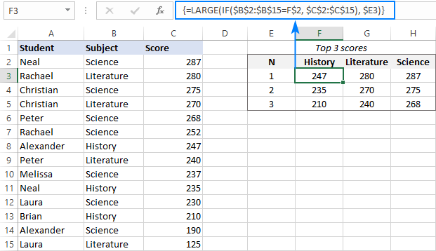
In the table below, supposing you want to find the biggest 3 scores in different subjects. To have it done, we input the subject names in separate cells (F2, G2 and H2), and then use this formula:
=LARGE(IF($B$2:$B$15=F$2, $C$2:$C$15), $E3)
Where B2:B15 is a list of subjects (criteria_range), C2:C15 are the scores (values), and E3 is n.
Of course, you can hardcode the subject name in the formula (e.g. $B$2:$B$15="Science"), but using a cell reference makes the solution more flexible.
The above formula goes to F3, and then you drag it 2 rows down and 2 columns to the right. Thanks to the skillful use of absolute and mixed cell references, the formula adjusts automatically when copied to other cells, letting you get all the results in one go!
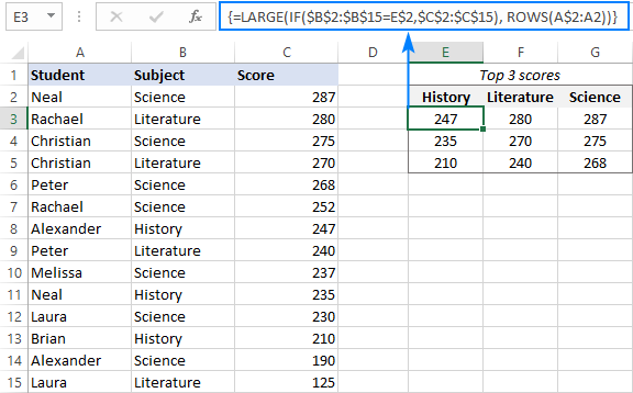
If needed, you can even do without typing n numbers on the sheet. Instead, generate them directly in the formula by embedding the ROWS function with an expanding range reference like this:
=LARGE(IF($B$2:$B$15=E$2,$C$2:$C$15), ROWS(A$2:A2))
The expanding range mechanics is explained in detail in this example, and here I will just show the result:
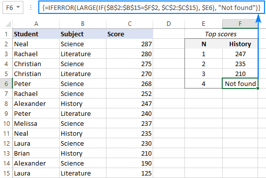
In case a specific largest value with a given condition is not found, the formula would return a #NUM! error. To prevent this from happening, wrap the LARGE IF formula inside the IFERROR function and replace the error with any value that you see fit, e.g. with a "-" or "Not found":
=IFERROR(LARGE(IF($B$2:$B$15=$F$2, $C$2:$C$15), $E3), "Not found")
How this formula works:
As you may know, the Excel LARGE function returns the n-th highest value specified in the 2nd argument from an array defined in the 1st argument. In our case, the array needs to be limited to only the scores in a given subject. To have it done, we embed an IF statement into the array argument, which compares each subject in B2:B15 with the target one in F2 (History):
IF($B$2:$B$15=$F$2, $C$2:$C$15)
Because IF performs the logical test on an array of numbers, the output is also an array, where the History scores are represented by numbers, and all other scores by FALSE values:
{FALSE;FALSE;FALSE;FALSE;FALSE;FALSE;247;FALSE;FALSE;235;FALSE;210;FALSE;FALSE}
The LARGE function ignores errors in the array and finds a specific n-th largest value among the History scores.
Excel LARGE IF with multiple criteria
To check several conditions in one formula, use one of the following methods:
Nest multiple IF statements one into another:
Multiply several range=criteria expressions:
In pre-dynamic Excel versions, both should be entered as array formulas by pressing Ctrl + Shift + Enter. In Excel 365, they can work as regular formulas as well.
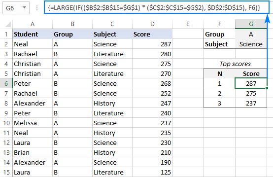
And now, let's try these techniques on our sample table. For this, we will add a new column, named Group, and use one of the below formulas to return top 3 scores in a given subject within a certain group:
=LARGE(IF($B$2:$B$15=$G$1, IF($C$2:$C$15=$G$2, $D$2:$D$15)), F6)
=LARGE(IF(($B$2:$B$15=$G$1) * ($C$2:$C$15=$G$2), $D$2:$D$15), F6)
Where:
- B2:B15 are the groups (criteria_range1)
- G1 is the target group (criteria1)
- C2:C15 is the list of subjects (criteria_range2)
- G1 is the target subject (criteria1)
- D2:D15 are the scores (values)
- F6 is n
Enter the formula in either one in G6 and copy it through G8. As the result, you will get the biggest 3 Science scores in group A.
When appropriate, you can put the criteria directly in the formula like this:
=LARGE(IF(($B$2:$B$15="A") * ($C$2:$C$15="Science"), $D$2:$D$15), F6)
But please remember this will require updating the formula each time the criteria change.
How these formulas work:
In the above formulas, we use the IF statements to test two different criteria, so only the values for which both conditions are TRUE make it into the LARGE function's array.
Formula 1 (nested IFs):
The logical test of the first IF statement compares the list of groups against the target one: $B$2:$B$15=$G$1. The result of the test is an array of TRUE and FALSE values, where TRUE's represent group A and FALSE any other group:
{TRUE;FALSE;TRUE;TRUE;FALSE;FALSE;TRUE;FALSE;TRUE;TRUE;FALSE;FALSE;TRUE;FALSE}
In a similar manner, the second IF compares the list of subjects with the target one (Science) and returns another TRUE and FALSE array:
{TRUE;FALSE;TRUE;FALSE;TRUE;TRUE;FALSE;FALSE;TRUE;FALSE;TRUE;FALSE;TRUE;FALSE}
For the items that have TRUE in both arrays, the nested IF formula returns the scores (value_if_true). The items that do not satisfy the criteria are represented by the FALSE values:
{287;FALSE;275;FALSE;FALSE;FALSE;FALSE;FALSE;237;FALSE;FALSE;FALSE;190;FALSE}
This final array is handed over to the LARGE function, from which it picks the n-th largest value.
Formula 2 (multiplying criteria):
In this formula, we evaluate two different criteria within a single logical test. The multiplication operation converts the logical values to 1's (TRUE) and 0's (FALSE). And because multiplying by 0 always gives zero, the resulting array has 1 for the items that meet both criteria:
{1;0;1;0;0;0;0;0;1;0;0;0;1;0}
The IF function evaluates this array 1's and 0's and passes the scores corresponding to 1's to LARGE.
LARGE IF formula with multiple criteria (OR logic)
To get the LARGE IF formula to work with the OR logic, i.e. when this or that condition is TRUE, sum the range=criteria expressions instead of multiplying them:
Supposing you want to find the largest 3 scores in two different subjects, say History and Literature. For Excel, you formulate the task differently: return the n-th largest score if Subject is either History OR Literature.
With criteria 1 (Literature) in F1 and criteria 2 (History) in F2, the formula goes as follows:
=LARGE(IF(($B$2:$B$15=$F$1) + ($B$2:$B$15=$F$2), $C$2:$C$15), E6)
Where B2:B15 are the subjects, C2:C15 are the scores, and E6 is the n-th largest value to return.
Complete the formula by pressing the Ctrl + Shift + Enter keys together, and you will get this result:
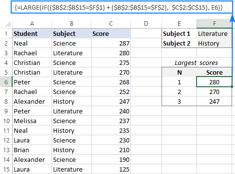
How this formula work:
In array formulas, the addition operation works like the OR operator:
The range=criteria expressions return two arrays of TRUE and FALSE values like those discussed in the previous example. After adding the elements of these arrays, we get an array of 1's and 0's, where 1's correspond to the items that meets either condition and 0's correspond to the items that do not meet any condition:
{0;1;0;1;0;0;1;1;0;1;0;1;0;1}
The IF function checks all the elements of the above array and hands off the scores corresponding to 1's to the LARGE function:
{FALSE;280;FALSE;270;FALSE;FALSE;247;240;FALSE;235;FALSE;210;FALSE;125}
FILTER top n values based on criteria
These solutions use a couple of dynamic array functions which are only available in Excel 356. In Excel 2019, Excel 2016 and earlier versions, these formulas won't work.
In Excel 365, there is one more way to get top N values with conditions. The beauty of this approach is that unlike traditional CSE array formulas the dynamic ones are completed in the usual way by pressing the Enter key. Moreover, the formula needs to be entered just in one cell and fills automatically across the entire spill range.
Formula 1. Filter top n values with one condition
To find the largest values based on condition, use this generic formula:
Where n is the number of top entries to extract.
For example, to get top 3 scores in a given subject, the formula in E4 is:
=SORT(FILTER(C2:C15, (C2:C15>=LARGE(IF(B2:B15=F1, C2:C15), 3)) * (B2:B15=F1)), 1, -1)
Where C2:C15 are the scores, B2:B15 are the subjects, and F1 is the subject of interest. Because the formula is entered just in one cell, you needn't bother about locking the ranges and cells with absolute references.
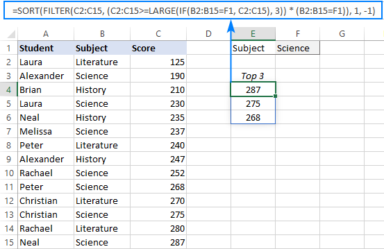
If you'd like to retrieve not only the scores but the related data as well, make the following adjustments to the formula:
- For the array argument of FILTER, supply the entire table (A2:C15).
- In the sort_index argument of SORT, indicate the number of the column to sort by (3rd column in our case).
=SORT(FILTER(A2:C15, (C2:C15>=LARGE(IF(B2:B15=F1, C2:C15), 3)) * (B2:B15=F1)), 3, -1)
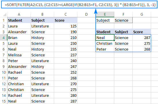
How this formula works:
The Excel FILTER function filters an array of data based on the criteria in the include argument. In our case, the criteria are as follows:
(C2:C15>=LARGE(IF(B2:B15=F1, C2:C15), 3)) * (B2:B15=F1))
The left part of the expression selects the scores that are greater than or equal to the 3rd highest score in the target group:
(C2:C15>=LARGE(IF(B2:B15=F1, C2:C15), 3))
Here, the IF function checks if the Subject is equal to the target one in F1 (Science) and passes the corresponding scores to LARGE. All other scores are replaced with FALSE:
{FALSE;190;FALSE;230;FALSE;237;FALSE;FALSE;252;268;FALSE;275;FALSE;287}
In the above array, the LARGE function finds the 3rd largest score, which is 268.
So, our criteria simplify to:
(C2:C15>=268) * (B2:B15=F1)
And the FILTER function resolves to:
FILTER(C2:C15, {0;0;0;0;0;0;0;0;0;1;0;1;0;1})
Where 1's correspond to scores greater than or equal to 268 in Science.
Finally, FILTER returns an array of top 3 scores:
{268;275;287}
The SORT function with the sort_order argument set to -1 arranges these scores in descending order and spills the results into E4:E6.
Formula 2. Filter top n values with multiple AND criteria
To filter the highest values with two or more conditions, you need to evaluate several logical expressions instead of one:
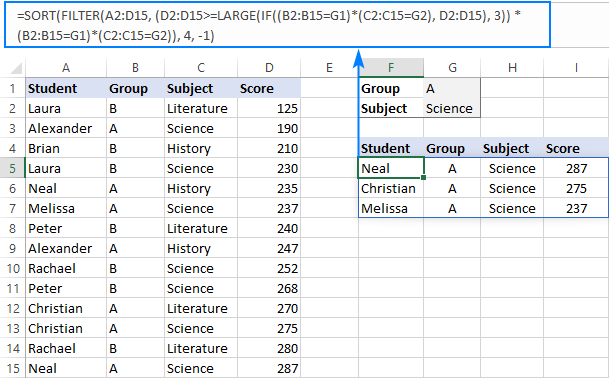
For example, to get top 3 scores among students of a particular group (G1) in a specific subject (G2), you could use this formula:
=SORT(FILTER(D2:D15, (D2:D15>=LARGE(IF((B2:B15=G1)*(C2:C15=G2), D2:D15), 3)) * (B2:B15=G1)*(C2:C15=G2)), 1, -1)
Where B2:B15 are the groups, C2:C15 are the subjects and D2:D15 are the scores.
To get the scores as well as the associated data, the formula in F5 is:
=SORT(FILTER(A2:D15, (D2:D15>=LARGE(IF((B2:B15=G1)*(C2:C15=G2), D2:D15), 3)) * (B2:B15=G1)*(C2:C15=G2)), 4, -1)
Formula 3. Filter top n values with multiple OR criteria
To evaluate several criteria using OR logic, we added up logical expressions in the LARGE IF formula. This approach works for the FILTER formula too:
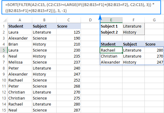
In our sample table, to retrieve top 3 scores in either Literature (F1) or History (F2), construct the criteria in this way:
=SORT(FILTER(C2:C15, (C2:C15>=LARGE(IF((B2:B15=F1)+(B2:B15=F2), C2:C15), 3)) * ((B2:B15=F1)+(B2:B15=F2))), 1, -1)
Where B2:B15 are the subjects and C2:C15 are the scores.
To extract not only the scores but all the related information, the formula in E5 is:
=SORT(FILTER(A2:C15, (C2:C15>=LARGE(IF((B2:B15=F1)+(B2:B15=F2), C2:C15), 3)) * ((B2:B15=F1)+(B2:B15=F2))), 3, -1)
FILTER n-th largest value with conditions
This solution only works in Excel 365. In other versions, the FILTER function is not available.
The previous examples show how to filter top N values with one or more conditions. If you need to find a specific value, say 2nd or 3rd highest number in a dataset, then you can use a much simpler LARGE FILTER formula.
The logic is basically the same as in LARGE IF formulas discussed in the first part of this tutorial. The difference is that you use the FILTER function instead of IF to apply the criteria.
Formula 1. Find n-th highest value with condition
For one condition, this basic formula will work:
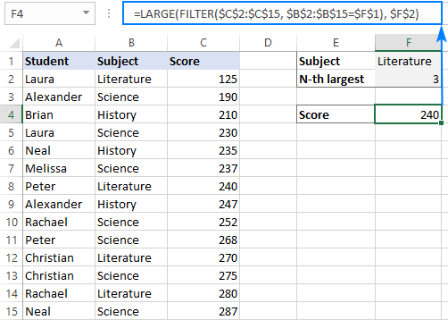
For example, to get the 3rd highest score in Literature, use one of these formulas:
=LARGE(FILTER($C$2:$C$15, $B$2:$B$15="Literature"), 3)
=LARGE(FILTER($C$2:$C$15, $B$2:$B$15=$F$1), $F$2)
Where B2:B15 are the subjects, C2:C15 are the scores, F1 is the subject of interest and F2 is the n-th largest score to return.
Formula 2. Filter n-th largest value using multiple AND criteria
To evaluate two or more criteria using the AND logic, here's the formula to use:
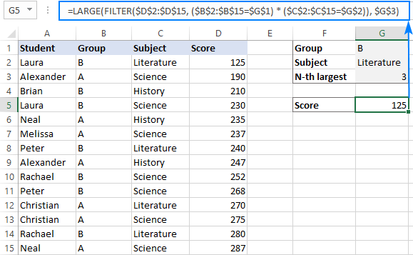
Supposing you are looking for the 3rd highest score (G3) in Literature (G2) in group B (G1). Supply the corresponding references to the formula:
=LARGE(FILTER($D$2:$D$15, ($B$2:$B$15=$G$1) * ($C$2:$C$15=$G$2)), $G$3)
And you will get this result:
Formula 3. Get n-th biggest value using multiple OR criteria
To test multiple criteria with the OR logic, the formula is:
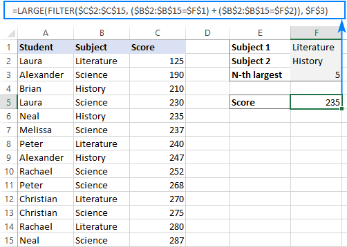
Let's say you wish to find the 5th highest score (F3) in humanitarian subjects - Literature (F1) or History (F2). The formula takes this shape:
=LARGE(FILTER($C$2:$C$15, ($B$2:$B$15=$F$1)+($B$2:$B$15=$F$2)), $F$3)
It will check if condition 1 or condition 2 is TRUE and output the result:
That's how to use Excel LARGE function with criteria. I thank you for reading and hope to see you on our blog next week!
Practice workbook for download
LARGE IF formula examples (.xlsx file)
 by
by
8 comments
What if you had a tie for second and you wanted to give the next highest to third?
Hi! If I understand your question correctly, then this article might be useful to you: Excel RANK functions with formula examples.
You can also try this formula:
=COUNT(1/FREQUENCY($A$2:$A$15,IF($A$2:$A$15>=A2,$A$2:$A$15)))
Hi,
What if i want the name of the student who is 1st, 2nd and 3rd by adding all marks in all subject.
Hi! If you use the sample data from paragraph: FILTER n-th largest value with conditions, then the problem can't be solved with a single formula. Get the list of unique student names using the UNIQUE function (for example, in column G)
=UNIQUE(A2:A15)
For each student, calculate the sum of the scores using the SUMIF function.
=SUMIF($A$2:$A$15,G1,$C$2:$C$15)
Find the maximum sum of the scores using the MAX function. Get the name of the student with the maximum sum of scores using INDEX MATCH.
=INDEX(G1:G10,MATCH(MAX(H1:H10),H1:H10,0))
I hope that the advice I have given you will help you solve your problem.
I'm using your formula from above:
=SORT(FILTER(A2:C15, (C2:C15>=LARGE(IF((B2:B15=F1)+(B2:B15=F2), C2:C15), 3)) * ((B2:B15=F1)+(B2:B15=F2))), 3, -1)
I don't want it to include the middle column in the results, but I everything I've tried to modify the formula doesn't seem to work. Any ideas?
Hi! I can assume that you want to show columns A and C as a result of the filter. Try using the CHOOSECOLS function to get some separate columns from the range. For example:
=SORT(FILTER(CHOOSECOLS(A2:C15,1,3), (C2:C15>=LARGE(IF((B2:B15=F1)+(B2:B15=F2), C2:C15), 3)) * ((B2:B15=F1)+(B2:B15=F2))), 3, -1)
I hope it’ll be helpful.
=(IF(LARGE($I$14:$AV$14,1)<0,"",(LARGE($I$14:$AV$14,1))))
i want to insert if error formula as well if the data is not available
Hello!
To avoid showing an error message, use the IFERROR function, as described in this guide: How to use IFERROR in Excel with formula examples.
=IFERROR(IF(LARGE($I$14:$AV$14,1)<0,"",(LARGE($I$14:$AV$14,1))),"")
This should solve your task.