 by
by Many tasks you perform in Excel involve comparing data in different cells. For this, Microsoft Excel provides six logical operators, which are also called comparison operators. This tutorial aims to help you understand the insight of Excel logical operators and write the most efficient formulas for your data analysis.
Excel logical operators - overview
A logical operator is used in Excel to compare two values. Logical operators are sometimes called Boolean operators because the result of the comparison in any given case can only be either TRUE or FALSE.
Six logical operators are available in Excel. The following table explains what each of them does and illustrates the theory with formula examples.
| Condition | Operator | Formula Example | Description |
| Equal to | = | =A1=B1 | The formula returns TRUE if a value in cell A1 is equal to the values in cell B1; FALSE otherwise. |
| Not equal to | <> | =A1<>B1 | The formula returns TRUE if a value in cell A1 is not equal to the value in cell B1; FALSE otherwise. |
| Greater than | > | =A1>B1 | The formula returns TRUE if a value in cell A1 is greater than a value in cell B1; otherwise it returns FALSE. |
| Less than | < | =A1<B1 | The formula returns TRUE if a value in cell A1 is less than in cell B1; FALSE otherwise. |
| Greater than or equal to | >= | =A1>=B1 | The formula returns TRUE if a value in cell A1 is greater than or equal to the values in cell B1; FALSE otherwise. |
| Less than or equal to | <= | =A1<=B1 | The formula returns TRUE if a value in cell A1 is less than or equal to the values in cell B1; FALSE otherwise. |
The screenshot below demonstrates the results returned by Equal to, Not equal to, Greater than and Less than logical operators:

It may seem that the above table covers it all and there's nothing more to talk about. But in fact, each logical operator has its own specificities and knowing them can help you harness the real power of Excel formulas.
Using "Equal to" logical operator in Excel
The Equal to logical operator (=) can be used to compare all data types - numbers, dates, text values, Booleans, as well as the results returned by other Excel formulas. For example:
| =A1=B1 | Returns TRUE if the values in cells A1 and B1 are the same, FALSE otherwise. |
| =A1="oranges" | Returns TRUE if cells A1 contain the word "oranges", FALSE otherwise. |
| =A1=TRUE | Returns TRUE if cells A1 contain the Boolean value TRUE, otherwise it returns FALSE. |
| =A1=(B1/2) | Returns TRUE if a number in cell A1 is equal to the quotient of the division of B1 by 2, FALSE otherwise. |
Example 1. Using the "Equal to" operator with dates
You might be surprised to know that the Equal to logical operator cannot compare dates as easily as numbers. For example, if the cells A1 and A2 contain the date "12/1/2014", the formula =A1=A2 will return TRUE exactly as it should.
However, if you try either =A1=12/1/2014 or =A1="12/1/2014" you will get FALSE as the result. A bit unexpected, eh?
The point is that Excel stores dates as numbers beginning with 1-Jan-1900, which is stored as 1. The date 12/1/2014 is stored as 41974. In the above formulas, Microsoft Excel interprets "12/1/2014" as a usual text string, and since "12/1/2014" is not equal to 41974, it returns FALSE.
To get the correct result, you must always wrap a date in the DATEVALUE function, like this =A1=DATEVALUE("12/1/2014")

Note. The DATEVALUE function needs to be used with other logical operator as well, as demonstrated in the examples that follow.
The same approach should be applied when you use Excel's equal to operator in the logical test of the IF function. You can find more info as well as a few formula examples in this tutorial: Using Excel IF function with dates.
Example 2. Using the "Equal to" operator with text values
Using Excel's Equal to operator with text values does not require any extra twists. The only thing you should keep in mind is that the Equal to logical operator in Excel is case-insensitive, meaning that case differences are ignored when comparing text values.
For example, if cell A1 contains the word "oranges" and cell B1 contains "Oranges", the formula =A1=B1 will return TRUE.
If you want to compare text values taking in to account their case differences, you should use the EXACT function instead of the Equal to operator. The syntax of the EXACT function is as simple as:
Where text 1 and text2 are the values you want to compare. If the values are exactly the same, including case, Excel returns TRUE; otherwise, it returns FALSE. You can also use the EXACT function in IF formulas when you need a case-sensitive comparison of text values, as shown in the below screenshot:

Note. If you want to compare the length of two text values, you can use the LEN function instead, for example =LEN(A2)=LEN(B2) or =LEN(A2)>=LEN(B2).
Example 3. Comparing Boolean values and numbers
There is a widespread opinion that in Microsoft Excel the Boolean value of TRUE always equates to 1 and FALSE to 0. However, this is only partially true, and the key word here is "always" or more precisely "not always" : )
When writing an 'equal to' logical expression that compares a Boolean value and a number, you need to specifically point out for Excel that a non-numeric Boolean value should be treated as a number. You can do this by adding the double minus sign in front of a Boolean value or a cell reference, e. g. =A2=--TRUE or =A2=--B2.
The 1st minus sign, which is technically called the unary operator, coerces TRUE/FALSE to -1/0, respectively, and the second unary negates the values turning them into +1 and 0. This will probably be easier to understand looking at the following screenshot:

Note. You should add the double unary operator before a Boolean when using other logical operators such as not equal to, greater than or less than to correctly compare a numeric and Boolean values.
When using logical operators in complex formulas, you might also need to add the double unary before each logical expression that returns TRUE or FALSE as the result. Here's an example of such a formula: SUMPRODUCT and SUMIFS in Excel.
Using "Not equal to" logical operator in Excel
You use Excel's Not equal to operator (<>) when you want to make sure that a cell's value is not equal to a specified value. The use of the Not equal to operator is very similar to the use of Equal to that we discussed a moment ago.
The results returned by the Not equal to operator are analogous to the results produced by the Excel NOT function that reverses the value of its argument. The following table provides a few formula examples.
| Not equal to operator | NOT function | Description |
| =A1<>B1 | =NOT(A1=B1) | Returns TRUE if the values in cells A1 and B1 are not the same, FALSE otherwise. |
| =A1<>"oranges" | =NOT(A1="oranges") | Returns TRUE if cell A1 contains any value other than "oranges", FALSE if it contains "oranges" or "ORANGES" or "Oranges", etc. |
| =A1<>TRUE | =NOT(A1=TRUE) | Returns TRUE if cell A1 contains any value other than TRUE, FALSE otherwise. |
| =A1<>(B1/2) | =NOT(A1=B1/2) | Returns TRUE if a number in cell A1 is not equal to the quotient of the division of B1 by 2, FALSE otherwise. |
| =A1<>DATEVALUE("12/1/2014") | =NOT(A1=DATEVALUE("12/1/2014")) | Returns TRUE if A1 contains any value other than the date of 1-Dec-2014, regardless of the date format, FALSE otherwise. |
Greater than, less than, greater than or equal to, less than or equal to
You use these logical operators in Excel to check how one number compares to another. Microsoft Excel provides 4 comparison operates whose names are self-explanatory:
- Greater than (>)
- Greater than or equal to (>=)
- Less than (<)
- Less than or equal to (<=)
Most often, Excel comparison operators are used with numbers, date and time values. For example:
| =A1>20 | Returns TRUE if a number in cell A1 is greater than 20, FALSE otherwise. |
| =A1>=(B1/2) | Returns TRUE if a number in cell A1 is greater than or equal to the quotient of the division of B1 by 2, FALSE otherwise. |
| =A1<DATEVALUE("12/1/2014") | Returns TRUE if a date in cell A1 is less than 1-Dec-2014, FALSE otherwise. |
| =A1<=SUM(B1:D1) | Returns TRUE if a number in cell A1 is less than or equal to the sum of values in cells B1:D1, FALSE otherwise. |
Using Excel comparison operators with text values
In theory, you can also use the greater than, greater than or equal to operators as well as their less than counterparts with text values. For example, if cell A1 contains "apples" and B1 contains "bananas", guess what the formula =A1>B1 will return? Congratulations to those who've staked on FALSE : )
When comparing text values, Microsoft Excel ignores their case and compares the values symbol by symbol, "a" being considered the lowest text value and "z" - the highest text value.
So, when comparing the values of "apples" (A1) and "bananas" (B1), Excel starts with their first letters "a" and "b", respectively, and since "b" is greater than "a", the formula =A1>B1 returns FALSE.
If the first letters are the same, then the 2nd letters are compared, if they happen to be identical too, then Excel gets to the 3rd, 4th letters and so on. For example, if A1 contained "apples" and B1 contained "agave", the formula =A1>B1 would return TRUE because "p" is greater than "g".

At first sight, the use of comparison operators with text values seems to have very little practical sense, but you never know what you might need in the future, so probably this knowledge will prove helpful to someone.
Common uses of logical operators in Excel
In real work, Excel logical operators are rarely used on their own. Agree, the Boolean values TRUE and FALSE they return, though very true (excuse the pun), are not very meaningful. To get more sensible results, you can use logical operators as part of Excel functions or conditional formatting rules, as demonstrated in the below examples.
1. Using logical operators in arguments of Excel functions
When it comes to logical operators, Excel is very permissive and allows using them in parameters of many functions. One of the most common uses is found in Excel IF function where the comparison operators can help to construct a logical test, and the IF formula will return an appropriate result depending on whether the test evaluates to TRUE or FALSE. For example:
=IF(A1>=B1, "OK", "Not OK")
This simple IF formula returns OK if a value in cell A1 is greater than or equal to a value in cell B1, "Not OK" otherwise.
And here's another example:
=IF(A1<>B1, SUM(A1:C1), "")
The formula compares the values in cells A1 and B1, and if A1 is not equal to B1, the sum of values in cells A1:C1 is returned, an empty string otherwise.
Excel logical operators are also widely used in special IF functions such as SUMIF, COUNTIF, AVERAGEIF and their plural counterparts that return a result based on a certain condition or multiple conditions.
You can find a wealth of formula examples in the following tutorials:
2. Using Excel logical operators in mathematical calculations
Of course, Excel functions are very powerful, but you don't always have to use them to achieve the desired result. For example, the results returned by the following two formulas are identical:
IF function: =IF(B2>C2, B2*10, B2*5)
Formula with logical operators: =(B2>C2)*(B2*10)+(B2<=C2)*(B2*5)

I guess the IF formula is easier to interpret, right? It tells Excel to multiply a value in cell B2 by 10 if B2 is greater than C2, otherwise the value in B1 is multiplied by 5.
Now, let's analyze what the 2nd formula with the greater than and less than or equal to logical operators does. It helps to know that in mathematical calculations Excel does equate the Boolean value TRUE to 1, and FALSE to 0. Keeping this in mind, let's see what each of the logical expressions actually returns.
If a value in cell B2 is greater than a value in C2, then the expression B2>C2 is TRUE, and consequently equal to 1. On the other hand, B2<=C2 is FALSE and equal to 0. So, given that B2>C2, our formula undergoes the following transformation:
![]()
Since any number multiplied by zero gives zero, we can cast away the second part of the formula after the plus sign. And because any number multiplied by 1 is that number, our complex formula turns into a simple =B2*10 that returns the product of multiplying B2 by 10, which is exactly what the above IF formula does : )
Obviously, if a value in cell B2 is less than in C2, then the expression B2>C2 evaluates to FALSE (0) and B2<=C2 to TRUE (1), meaning that the reverse of the described above will occur.
3. Logical operators in Excel conditional formatting
Another common use of logical operators is found in Excel Conditional Formatting that lets you quickly highlight the most important information in a spreadsheet.
For example, the following simple rules highlight selected cells or entire rows in your worksheet depending on a value in column A:
Less than (orange): =A1<5
Greater than (green): =A1>20

For the detailed-step-by-step instructions and rule examples, please see the following articles:
As you see, the use of logical operators in Excel is intuitive and easy. In the next article, we are going to learn the nuts and bolts of Excel logical functions that allow performing more than one comparison in a formula. Please stay tuned and thank you for reading!
1250 comments
I have one problem please help me
i have 2 value cell D6 value & E6
if value D6 >= E6+(E6*0.5%) answer is E6
if value D6 <=E6-(E6*0.5%) answer is E6
if value D6 < E6-(E6*0.5%) answer is S6
thanks & regards
Niranjan
I have the following formula and Excel continues to give me errors. Help, please!
=IF(B126>20,"A",IF(AND(B126=0),"B",IF(AND(B126(-20)), "C"), IF(B126<(-20), "D")))
Hello, Matthew,
first of all, you don't need to use AND function because you specify only one criterion after it. Then, you missed the logical operator in B126(-20): should B126 be equal to -20? Also, there's no need to use round brackets for negatives in this case.
So, try this formula:
=IF(B126>20,"A",IF(B126=0,"B",IF(B126=-20,"C",IF(B126<-20,"D")))) Please note that you didn't specify what to return when B126<0 but greater than -20; when B126=20 and when B126>0 but lower than 20. Logically the formula requires these criteria too.
But I do hope that the formula above is what you were looking for :)
Hi Svetlana,
Scenario:
F8 = 1
D10 = 0
E10 = 7
I want to create an IF formula to ask if F8 is greater than D10 but less than E10, then return a value of 1. If not, then return a blank.
I created the following:
IF(F8>D10<=E10,1,"")
but this returns a blank instead of 1. I am not sure why.
I am sure it is probably quite simple, but can't seem to solve it - I would be grateful for your help.
Many thanks!
Hi Aron,
you need to use AND in the condition of your formula. Try the following:Excel IF tutorial.
=IF(AND(F8>D10,F8
Hi,
I have a problem if somebody can help me it would be very appreciable. I had wrote many formula but did not get results.
We have data like:
Age Actual Value Exempted Value
50 30000
50 14500
50 25000
60 30000
60 19100
60 35000
We want to get results:
Age Actual Value Exempted Value
50 30000 25000
50 14500 14500
50 25000 25000
60 30000 30000
60 19100 19100
60 35000 30000
Note: There are upper cap for 25000 60
Hi,
Need help on this'
1-24 = A
25-30 = b
31-48 = c
This is my formula but not working
=IF(A1=25,A1=31,"C")))
many thanks,
necie
Hi Guys
some one help me for fixing up this issue,
formula for:-
If the amount is less than 50,00,000 then its 0%, if the amount is between 50 lakhs and 1 cr its 10% and above 1 cr its 15%.
Hi can someone help me in this.
I need to add numbers between given two numbers
Eg.
if I give first number 18 and last number 20 in different cell
the number should generate Automatically in this sequence
18.25
18.50
18.75
19.00
19.25
19.50
19.75
20.00
the sequence should stop to given last number.
please help me out
thank you
Hi,
Can someone assist me with the following request please.
In Column A1, if someone types or pull the following hours of data from the list (8,16,24,32,40,48,56,64,72). The max is 72 hours.
Column B1 should provide the following:
1. Remaining hours left
Column C1 should provide the following:
1. Percentage of hours left from 100%
2. Color scales of stop light (Green, Yellow, Red)
I hope that I was able to make a sense of my request! Thank you in advance!
I am seeking assistance on a formula: If C3-B3 is greater than 51% then E14 is C3-B3*.10
If 100-35 > 51, then 65*.10
Thank you in advance!
Hello,
I'm trying to setup a formula within the conditional formatting. If i have two cells that have the same name in them, then I'm hoping to have the conditonal formatting kick in and shade the a cell a certain color. Where I get stuck is getting the formula to refer to the conditional formatting instead of giving me a text output as the result.
For example, =IF(AND(A1=Bob,A2=Bob),X,X) Where X represents the instruction to shade or not shade a cell.
I know I can put a formula in a conditional format rule but not sure how to make the true/false variables refer to the shading.
Any advise/help would be appreciated!
Thanks,
Corey
The formula is:
IF((D3="Men"),(E11>19,E1115,E11<25),RED,NO FILL)
Thanks for help provided.
John
i have a sheet with a drop down list of "Men" and "Women". i have put the following IF formula based on the criteria of BMR between the range for Men >19 but 15 but 19,E1115,E11<25),RED,BLUE)
I am getting all wrong somewhere. Please rectify the same.
Thanks in advance.
John Sanil
I have a question. I'm trying to work out a formula where, if a figure (A) is lower than a figure range it will equal YES. And if a figure (A) is greater than figure range it will equal NO
Figure range
1 to 12
1 to 24
1 to 36
1 to 120
1 to 240
example: IF (A) is between 1 to 12 = YES, greater than 12 = NO
I hope this makes some sort of sense and you can help.
=IF(AND(G3>=$C$3,G3<=$D$3),"Pass","Fail")
I want to be able to Round both the Less than or Equal to value and the Greater than or equal to value. I want to be able to Round the greater than or equal to value up and and the less than or equal to down. Every time I try and add rounding to the above formula I get errors.
Example Nominal Low Tol. Upper Tol. Act. Act. Form.Above
PD Go Top 0 deg. 27.735 27.735 27.747 27.7471 27.747 Fail
Help! I trying to find if cell A1 is equal to B1 and if it is highlight it a secific color, red. There are about 15k so I'll need to drag the formula down. Please help!
Hello, Anna,
if I understand your task correctly and you need to fill the cells with a colour depending on the result of the formula, then conditional formatting is what you need to take a look at.
You create the following rule:
=$A1=$B1
and apply it to
=$A:$B
Hope this helps.
Hi,
I am trying to apply a formula that returns a Text answer to the greater or less than number difference compared to an adjacent cell.
The purpose is for a 14 question questionnaire with either an A. or B. answer. The answer is determined by the criteria as follows:
"To score your test, add the number of questions you answered A and the
number you answered B"
- If your number of A answers is 3 or more than B answers, you are a
Protein Type.
- If your number of A and B answers are tied or within 2 of each other, you
are a Mixed Type.
- If your number of B answers is 3 or more than A answers, you are a
Carbohydrate Type.
I would like to return the text either "Protein Type", "Carb Type", "Mixed Type" based on the A. and B. totals.
Many Thanks
Hi Brad,
Let's assume that your data is arranged in the following way:
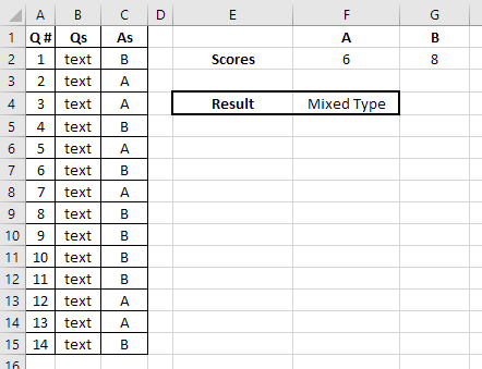
A1:C15 is the table with questions (Qs) and answers (As).
Using COUNTIF in F2 and G2 we can find out the number of 'A' and 'B' answers accordingly:
=COUNTIF(C2:C15,"A") (for F2)
=COUNTIF(C2:C15,"B") (for G2)
Then, in F4 we need to use nested IF function to apply all the conditions you described:
=IF((F2-G2)>=3, "Protein Type", IF(AND((F2-G2)<=2,(F2-G2)>=-2),"Mixed Type","Carb Type"))
or a bit shorter version:
=IF((F2-G2)>=3, "Protein Type", IF(ABS(F2-G2)<=2,"Mixed Type","Carb Type"))
Try to adjust this example formulas to your data, and learn more on the used functions from the links above. Hope it helps!
Hi
I am trying to write a formula to colour code some values by looking at a formula. If the value is higher than the target it should print P, if it is equal to the target G and if it is within 90% of the target A and below 90% of target R. I have it working for some values but not for others.
eg the target is 0.4 - students made 0.4 progress so it should go green but it is going Amber. The 0.4 is calculated from another formula. If I type 0.4 then it goes green. I'm not sure what is going wrong.
Any help greatly appreciated.
Hi, Sarah,
could you send us a workbook sample with the data you use and the result you expect to get to support@ablebits.com? If it's impossible, then open your 'Conditional Formatting Rules Manager' and make sure that Stop If True box is checked for every rule you created.
Hello everyone
Kindly help me out as today i was trying to find out some.i can explain you by an example
Column A
2.5
2.8
2.7
2.44
2.32
1.8
3.2
I want to put them in two different column
Column 1- Value upto 2.5 but if less than 2.5 then put the lower value means if we select 1.8 then result will b 1.8
Column 2 - value which is greater then 2.5 but after deduction of 2.5 mean if we select 3.2 then the result will be 0.7
Please HELP...
im not so familiar using TRUE and FALSE, but i want to know more.
example i have a constant value of 10,000.
i want to know if [cell[A1] 5,000 ] is lesser than [cell[B1] 10,000, and [cell[B1] 10,000 is lesser than [cell[C1] 20,000.
i made this formula, please correct me.
= if(A1<B1<C1, "false","true")
then, if i change the constant value [cell[B1] to be 1,000] the answer must be "FALSE".
how to make this right? my answer always "TRUE" though i change the constant value at cell[B1] to a lesser value.
i know this is wrong, but please correct me, what it should exactly be.
THANKS..
You need to add AND function into your formula for multiple conditions. Try using the following:
=IF(AND(A1<B1, B1<C1),"true","false")
Hi,
I'm having the same problem, only I'm trying to determine a "True","False" outcome for numbers different by a specific amount. How do I write the above solution to include a specific difference. Eg: If A1 is different than B1 by 3 or more then "Text A", but B1 is different by 3 then "Text B". If they A1 and B1 are within a difference of 2 then "Text C".
I have posted a comment below, but found it difficult to explain myself properly.
Many Thanks
Hi Brad,
If my understanding of the task is correct, the following formula should work a treat:
=IF(A1-B1>=3,"text A",IF(B1-A1>=3,"text B","text C"))
If a1 is 40 b1 should be 40 if a1 is 50 b1 should be 50 if a1 is 60 b1 should be 50 kinly send a formula
Hi guys,
How can i create a formula in google spreadsheet if the scenario is this:
I would like to filter per quarter the regularization anniversary of our employees like this
Regularization date example Mar 3, 2017
i want to get the 4th quarter which is October to november
if the regularization date is in October to November it must say Yes, if not NO and N/A.
Please help me
let me know your thought about this.
Thanks
Jomarie
I have a spreadsheet which calculates the time in, time out, and lunch time, giving me a total of working time.
Example below:
7:54 AM 12:00 PM 12:30 PM 2:32 PM 6.13 1.87
A1 B1 C1 D1 E1 F1
Spreadsheet work great for A1 to E1, the problem that I have is F1, I need a maximum number there of no more the 2.0, and for the life of me I can't figure out the formula.
Example that is there now. =IF(A1>0, 8-E1)
Can anyone help me out how to figure the formula so that F1 can only equal up to 2.0 or less.
Thanks, Tammy
The score - 21-16 = 5, 16 - 21 = -5 ok but I would like to put "D" instead of blank when the score is draw (21-21)
Thanks in advance
If cell a has 5 and cell b has 4 I want to know if cell a is greater then cell b …….BUT only if it is only great then 1
Hi everybody,
I am using a simple Excel function
IF(A5=B5,"OK","False")
up to a certain amount it says OK but if the amount of A5 and B5 goes above a certain amount it says False although they are the same.
For examole:
A5=500 B5=500 OK
A5=600 B5=600 False
A5=700 B5=700 OK
Hello Mam,
I would like to know how to formula for date value is equal or greater than or less then in two cells.
example:
03/04/2017 03/04/2017 true
03/04/2017 03/04/2017 true
03/03/2017 03/04/2017 greater than
03/06/2017 03/04/2017 Less than
03/05/2017 03/04/2017 Less than
03/08/2017 03/03/2017 Less than
Hi, Need help!
If Cell A is grater or less than cell B by 10 units say "check" if not say "ok"
So would look like:
if A1 = 42 and B1= 42 then "OK"
if A1=53 and B1=42 then "check"
if A1 = 31 and B1 = 42 then "check"
Greetings,
Can someone explain to me how I would interpret this?
I understand the TEXT and the RIGHT syntax, but how are the 4 cells being compared? What is the result?
=TEXT(RIGHT(F12,2)>RIGHT(F21,2)>RIGHT(F32,2)>RIGHT(F41,2))
Thank you!
I need a solution for this
I want to add 1 to cell h1 if value in cell k11:k2000 is greater than 0.
Can we apply a formula greater than equal to when i have dates in two different rows.
Hi
Im looking for a formula that if
A2 or A3 are less than or equal to 3 but also greater than or equal to 1, D8 will equal 125. If either one is greater than 3, it will equal 0.
Please help :) Thank you
Hello,
I need help with a formula. I need it to say the following
If SUM A1:A15 >= 20,000 Then return 5% of SUM A1:A15
If 10,000 <= SUM A1:A15 < 20,000 return 4% of SUM A1:A15
If SUM A1:A15 < 10,000 return 3% of sum
How do I do this???
Hi
I need formula if I travel >=100 kms, it should calculate as Rs 600, If it's <100Kms it should consider Rs 350, please help
Hi there! I'm trying to do what I thought was something simple. I have a column that has 4 possible text inputs: T1, T2, T3, T4. I want the cell to be red if the text is either T3 or T4. How do I set that up? I can easily do conditional formatting if I use just *one* text input, but I can't figure out how to do it with an OR operator. I appreciate any guidance, from anyone!
Hi Svetlana
Can you help?
If CELL A1 is greater than Value 75, show Value 4.50
Any ideas?
Many thanks in advance.
Hi
Need a formula
if we cosider 3 cells A1, B1, C1
lets suppose c1=100
i want to have A1+B1=100(c1) all the time
if i change A1 to 60 then B1 should automatically display 40
and if i change B1 to 30 then A1 should automatically change to 70.
please help me out.
Hi
Please help. How to make condition monitoring with 2 conditons:
Column Z5 = RELMNC (text)
Column AA5 = 10 (number)
In column AA5 I want :
if left Z5;3 = "REL" , then value >=7, color fill Red
if left Z5;3 = "REL" , then value <=7, color fill Green
Thank you.
1 A B C D
2 Date1 Date2 Date3 Date4
3 1/23/2017 1/22/2017 1/21/2017 1/20/2017
I want to retrieve the status if A>B, B>C, C>D, "OK", ELSE "NOT OK"
PLEASE HELP ON THIS.
by using excel work sheet
I have the question;
how to calculate attendance percentage of student who sit to all course assessment and semester exam
want a formula for .
if A >= B , IN 90 DAYS , THEN GOOD OR BAD .
PLEASE SOME 1 CAN HELP PUT THIS IN A FORMULA .
REGARDS,
MARK
Hi Svetlana,
If I wanted to perform a mathematical function on a "<" less than number, what would I enter for the formula? e.g. <0.5 * 0.002 = <0.001
A B
1 0
-1 0
0 0
13 1
5 0.5
I need the usage of if condition like above answer
if less than 5 = 0
if greater than 5 and less than 13 = .5
if equal to 13 = 1
Hello,
I have some Amount like as 20,50,70,100,1000,2000,5000,10000. I am calculating with 10% for each data,but i want (%) value will not less than 10 and not more than 100. How can it possible?
Hi,
How to write in if formula that a cell is greater than 31/12/2015 and less than 01/01/2017. I can't use IF(AND function because I already used AND function for another argument. Or is there any way to specify a particular time period in IF function?
Thanks in advance.
Bharat
Hello,
I have a little problem. I have the following formula:
=COUNTIFS(Doigahama!H5:H214,"=0",Doigahama!P5:P214, ">=0")
However, the result I get is as if formula said only
=COUNTIFS(Doigahama!H5:H214,"=0",Doigahama!P5:P214, "=0")
The > is ignored. If I change the order of the signs to =>, then the = is ignored and I get only the values over, but not including 0. How can I fix this? I was searching for advice, but everywhere I look it seemed that the way to write greater or equal was like that.
Just in case i also tried using ≥, which did not work either, it was not recognised at all.
Any advice would be welcomed.
I am using Office 2010 with Windows 7.
Thank you,
Sincerely,
Florencia
Hi Svetlana,
Need a formula based on below criteria:
I have two cells, A and B,
if the difference btw A & B is less than 6 or equal to 6, "No Change"
if greater than 6 and less than 9, "Slight Change"
if greater than 10 "Significant Change"
Also the formula should override the difference with positive numbers, even the B is larger than A, vice-versa
Please help!!
Reply
Hi Svetlana,
Need a formula based on below criteria:
I have two cells, A and B,
if the difference btw A & B is below 6 or equal to 6, "No Change"
if above 6 and below 9, "Slight Change"
if above 10 "Significant Change"
Also the formula should override the difference with positive numbers, even the B is larger than A, vice-versa
Please help!!
Hi, i need help...is there a formula where i can add a number if a cell is bigger than another cell by a certain number EXAMPLE...
if A is greater than B by 2 then add 3, if A is greater than B by 3 then add 5
Also is there a formula where if C contains "draw" add 1, if C contains "win" add 2
Hi,
i want automatic sort out the all values less then 9.8 an other sell. so plz tell about formula.
thanks