The tutorial explains how to use COUNTIFS and COUNTIF formulas with multiple criteria in Excel based on AND as well as OR logic. You will find a number of examples for different data types - numbers, dates, text, wildcard characters, non-blank cells and more.
Of all Excel functions, COUNTIFS and COUNTIF are probably most often mixed up because they look very much alike and both are purposed for counting cells based on the specified criteria.
The difference is that COUNTIF is designed for counting cells with a single condition in one range, whereas COUNTIFS can evaluate different criteria in the same or in different ranges. The aim of this tutorial is to demonstrate different approaches and help you choose the most efficient formula for each particular task.
Excel COUNTIFS function - syntax and usage
The Excel COUNTIFS function counts cells across multiple ranges based on one or several conditions. The function is available in Excel 365, 2021, 2019, 2016, 2013, Excel 2010, and Excel 2007, so you can use the below examples in any Excel version.
COUNTIFS syntax
The syntax of the COUNTIFS function is as follows:
- criteria_range1 (required) - defines the first range to which the first condition (criteria1) shall be applied.
- criteria1 (required) - sets the condition in the form of a number, cell reference, text string, expression or another Excel function. The criteria defines which cells shall be counted and can be expressed as 10, "<=32", A6, "sweets".
- [criteria_range2, criteria2]… (optional) - these are additional ranges and their associated criteria. You can specify up to 127 range/criteria pairs in your formulas.
In fact, you don't have to remember the syntax of the COUNTIF function by heart. Microsoft Excel will display the function's arguments as soon as you start typing; the argument you are entering at the moment is highlighted in bold.

Excel COUNTIFS - things to remember!
- You can use the COUNTIFS function in Excel to count cells in a single range with a single condition as well as in multiple ranges with multiple conditions. If the latter, only those cells that meet all of the specified conditions are counted.
- Each additional range must have the same number of rows and columns as the first range (criteria_range1 argument).
- Both contiguous and non-contiguous ranges are allowed.
- If the criteria is a reference to an empty cell, the COUNTIFS function treats it as a zero value (0).
- You can use the wildcard characters in criteria - asterisk (*) and question mark (?). See this example for full details.
How to use COUNTIFS and COUNTIF with multiple criteria in Excel
Below you will find a number of formula examples that demonstrate how to use the COUNTIFS and COUNTIF functions in Excel to evaluate multiple conditions.
How to count cells with multiple criteria (AND logic)
This scenario is the easiest one, since the COUNTIFS function in Excel is designed to count only those cells for which all of the specified conditions are TRUE. We call it the AND logic, because Excel's AND function works this way.
Formula 1. COUNTIFS formula with multiple criteria
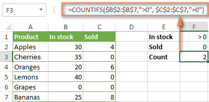
Suppose you have a product list like shown in the screenshot below. You want to get a count of items that are in stock (value in column B is greater than 0) but have not been sold yet (value is column C is equal to 0).
The task can be accomplished by using this formula:
=COUNTIFS(B2:B7,">0", C2:C7,"=0")
And the count is 2 ("Cherries" and "Lemons"):
Formula 2. COUNTIFS formula with two criteria
When you want to count items with identical criteria, you still need to supply each criteria_range / criteria pair individually.
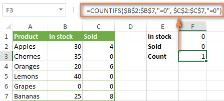
For example, here's the right formula to count items that have 0 both in column B and column C:
=COUNTIFS($B$2:$B$7,"=0", $C$2:$C$7,"=0")
This COUNTIFS formula returns 1 because only "Grapes" have "0" value in both columns.
Using a simpler formula with a single criteria_range like COUNTIFS(B2:C7,"=0") would yield a different result - the total count of cells in the range B2:C7 containing a zero (which is 4 in this example).
How to count cells with multiple criteria (OR logic)
As you have seen in the above examples, counting cells that meet all of the specified criteria is easy because the COUNTIFS function is designed to work this way.
But what if you want to count cells for which at least one of the specified conditions is TRUE, i.e. based on the OR logic? Overall, there are two ways to do this - by adding up several COUNTIF formulas or using a SUM COUNTIFS formula with an array constant.
Formula 1. Add up two or more COUNTIF or COUNITFS formulas
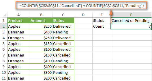
In the table below, supposing you want to count orders with the "Cancelled" and "Pending" status. To have it doen, you can simply write 2 regular Countif formulas and add up the results:
=COUNTIF($C$2:$C$11,"Cancelled") + COUNTIF($C$2:$C$11,"Pending")
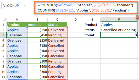
In case each of the functions is supposed to evaluate more than one condition, use COUNTIFS instead of COUNTIF. For example, to get the count of "Cancelled" and "Pending" orders for "Apples" use this formula:
=COUNTIFS($A$2:$A$11, "Apples", $C$2:$C$11,"Cancelled") + COUNTIFS($A$2:$A$11, "Apples", $C$2:$C$11,"Pending")
Formula 2. SUM COUNTIFS with an array constant
In situations when you have to evaluate a lot of criteria, the above approach is not the best way to go because your formula would grow too big in size. To perform the same calculations in a more compact formula, list all of your criteria in an array constant, and supply that array to the criteria argument of the COUNTIFS function. To get the total count, embed COUNTIFS inside the SUM function, like this:
In our sample table, to count orders with the status "Cancelled" or "Pending" or "In transit", the formula would go as follows:
=SUM(COUNTIFS($C$2:$C$11, {"cancelled", "pending", "in transit"}))
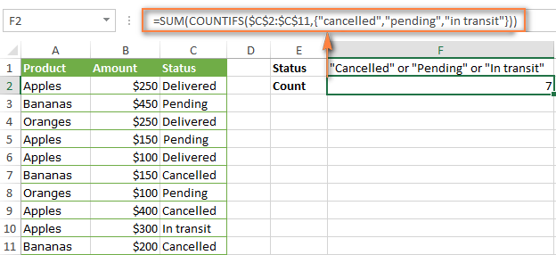
In a similar manner, you can count cells based on two or more criteria_range / criteria pairs. For instance, to get the number of "Apples" orders that are "Cancelled" or "Pending" or "In transit", use this formula:
=SUM(COUNTIFS($A$2:$A$11,"apples",$C$2:$C$11,{"cancelled","pending","in transit"}))

You can find a few more ways to count cells with OR logic in this tutorial: Excel COUNTIF and COUNTIFS with OR conditions.
How to count numbers between 2 specified numbers
By and large, COUNTIFS formulas for numbers fall into 2 categories - based on several conditions (explained in the above examples) and between the two values you specify. The latter can be accomplished in two ways - by using the COUNTIFS function or by subtracting one COUNTIF from another.
Formula 1. COUNTIFS to count cells between two numbers
To find out how many numbers between 5 and 10 (not including 5 and 10) are contained in cells C2 through C10, use this formula:
=COUNTIFS(C2:C10,">5", C2:C10,"<10")
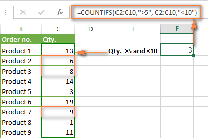
To include 5 and 10 in the count, use the "greater than or equal to" and "less than or equal to" operators:
=COUNTIFS(B2:B10,">=5", B2:B10,"<=10")
Formula 2. COUNTIF formulas to count numbers between X and Y
The same result can be achieved by subtracting one Countif formula from another. The first one counts how many numbers are greater than the lower bound value (5 in this example). The second formula returns the count of numbers that are greater than the upper bound value (10 in this case). The difference between the first and second number is the result you are looking for.
- =COUNTIF(C2:C10,">5")-COUNTIF(C2:C10,">=10") - counts how many numbers greater than 5 and less than 10 are in the range C2:C10. This formula will return the same count as shown in the screenshot above.
- =COUNTIF(C2:C10, ">=5")-COUNTIF(C2:C10, ">10") - the formula counts how many numbers between 5 and 10 are in the range C2:C10, including 5 and 10.
How to use cell references in COUNTIFS formulas
When using logical operators such as ">", "<", "<=" or ">=" together with cell references in your Excel COUNTIFS formulas, remember to enclose the operator in "double quotes" and
add an ampersand (&) before a cell reference to construct a text string.
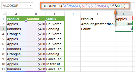
In a sample dataset below, let's count "Apples" orders with amount greater than $200. With criteria_range1 in cells A2:A11 and criteria_range2 in B2:B11, you can use this formula:
=COUNTIFS($A$2:$A$11, "Apples", $B$2:$B$11, ">200")
Or, you can input your criteria values in certain cells, say F1 and F2, and reference those cells in your formula:
=COUNTIFS($A$2:$A$11, $F$1, $B$2:$B$11, ">"&$F$2)
Please notice the use of absolute cell references both in the criteria and criteria_range arguments, which prevents the formula from being broken when copied to other cells.
For more information about the use of an ampersand in COUNTIF and COUNTIFS formulas, please see Excel COUNTIF - frequently asked questions.
How to use COUNTIFS with wildcard characters
In Excel COUNTIFS formulas, you can use the following wildcard characters:
- Question mark (?) - matches any single character, use it to count cells starting and/or ending with certain characters.
- Asterisk (*) - matches any sequence of characters, you use it to count cells containing a specified word or a character(s) as part of the cell's contents.
Tip. If you want to count cells with an actual question mark or asterisk, type a tilde (~) before an asterisk or question mark.
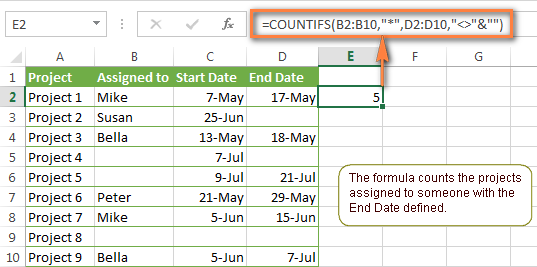
Now let's see how you can use a wildcard char in real-life COUNTIFS formulas in Excel. Suppose, you have a list of projects in column A. You wish to know how many projects are already assigned to someone, i.e. have any name in column B. And because we are learning how to use the COUNTIFS function with multiple criteria, let's add a second condition - the End Date in column D should also be set.
Here is the formula that works a treat:
=COUNTIFS(B2:B10,"*",D2:D10,"<>"&""))
Please note, you cannot use a wildcard character in the 2nd criteria because you have dates rather that text values in column D. That is why, you use the criteria that finds non-blank cells: "<>"&""
COUNTIFS and COUNTIF with multiple criteria for dates
The COUNTIFS and COUNTIF formulas you use for dates are very much similar to the above formulas for numbers.
Example 1. Count dates in a specific date range
To count the dates that fall in a certain date range, you can also use either a COUNTIFS formula with two criteria or a combination of two COUNTIF functions.
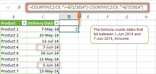
For example, the following formulas count the number of dates in cells C2 through C10 that fall between 1-Jun-2014 and 7-Jun-2014, inclusive:
=COUNTIFS(C2:C9, ">=6/1/2014", C2:C9, "<=6/7/2014")
=COUNTIF(C2:C9, ">=6/1/2014") - COUNTIF(C2:C9, ">6/7/2014")
Example 2. Count dates with multiple conditions
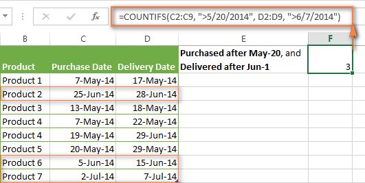
In the same manner, you can use a COUNTIFS formula to count the number of dates in different columns that meet 2 or more conditions. For instance, the below formula will find out how many products were purchased after the 20th of May and delivered after the 1st of June:
=COUNTIFS(C2:C9, ">5/1/2014", D2:D9, ">6/7/2014")
Example 3. Count dates with multiple conditions based on the current date
You can use Excel's TODAY() function in combination with COUNTIF to count dates based on the current date.
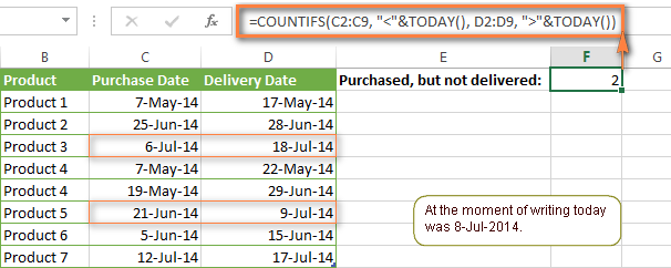
For example, the following COUNTIF formula with two ranges and two criteria will tell you how many products have already been purchased but not delivered yet.
=COUNTIFS(C2:C9, "<"&TODAY(), D2:D9, ">"&TODAY())
This formula allows for many possible variations. For instance, you can tweak it to count how many products were purchased more than a week ago and are not delivered yet:
=COUNTIFS(C2:C9, "<="&TODAY()-7, D2:D9, ">"&TODAY())
This is how you count cells with multiple criteria in Excel. I hope you will find these examples helpful. Anyway, I thank you for reading and hope to see you on our blog next week!
 by
by
1979 comments
Having Issues with a Count IF, I was wondering if you could help. I want to Count if there is date in Cell and if another column reads not released.
=COUNTIF('Development '!E3:E52,"",'Development '!E3:E100","Not Released")
Hi Sean,
Try the following formula:
=COUNTIF('Development '!E3:E52,"")+COUNTIF('Development '!E3:E100","Not Released")
Hi,
May I have support from you guys,
this function is not working: =COUNTIFS(C:C,"=CW17",J8:L103,"=Customer not available")!!!!!!!!!!
C:C= is a criteria range contain Calendar weeks
J8:L103= I need to count a criteria " Customer not available"
when I Enter that function, I get this answer= #Value!
Please please assist me.
Best.
Hi, I wish to count the number of cells that say "yes" in column A relating to the date between a certain range, ie: 01/10/2015 to the 31/10/2015 in column B so for example if I have 10 people who say yes in Oct on specific dates in October, it would read 10 in the results call. I am currently using this formula:
=COUNTIFS(G5:G12,"=Nov",H5:H12,"=Yes")
but I don't know how to pick up the result then reading cells with specific dates, ie: 20/11/2015. I want to pick up the result between the 1st Nov and the 3th Nov.
Can anyone help please?
Hi
Value in cell A3 is 10
I want to check this value tn 4 Different Criteria
1)Less than 20
2)Greater than 20 but less than 50
3)Greater than 50 but less than 80
4)greater than 80
Please help
Regards
Venkat
I have 2 columns of data. I would like to count the number of cells where column 1 is greater than column 2. I imagined something like this: =COUNTIF(G17:G50,">C7:C38") But that does not work. Suggestions? Thanks.
Hello Dave,
To compare ranges, you can use an array Sum formula similar to this (completed by pressing Ctrl+Shift+Enter):
=SUM(--(G17:G50>C17:C50))
Please pay attention that the ranges should be of the same size, i.e. include the same number of rows.
what is the formula if I want to get the total number of invoice issued per saleperson and categories by date, like from Jan, Feb, March etc. for the whole year.
thank you!
I have cells with multiple data separated by commas, How to use countif or countifs fuction on this data. Like the student name has multiple student1,student 2etc separted by commas. How to use countif on them.
Lecturer Name Subject Student Names
Dr Raj Gross Anatomy Lecture Student 1, Student 3,
Dr Sreekanth Gross Anatomy Lecture Student 1, Student 2, Student 3, Student 5, Student 6
Dr Hannah Histology Lecture Student 1
Dr Stella Anatomy Lab Student 1, Student 2, Student 3, Student 4, Student 5, Student 6
Please I am on this table too.
Mine is about cells with multiple years entered n separated by commas.
How do I count cells that contain only two of the many years entered in no particular order?
Dear Svetlana
I have cells with multiple data separated by commas, How to use countif or countifs fuction on this data. Like the student name has multiple student1,student 2etc separted by commas. How to use countif on them.
Lecturer Name Subject Student Names
Dr Raj Gross Anatomy Lecture Student 1, Student 3,
Dr Sreekanth Gross Anatomy Lecture Student 1, Student 2, Student 3, Student 5, Student 6
Dr Hannah Histology Lecture Student 1
Dr Stella Anatomy Lab Student 1, Student 2, Student 3, Student 4, Student 5, Student 6
what is the formula if I want to get the number of invoice issued per saleperson and categories by date, like from Jan, Feb, March etc. the whole year.
thank you!
how do I add numbers if a certain product is beside it
a1 b1
200 161
300 NC
900 2100
I want to be able to automatically add a1 if the square contains one of the products in B1 -how do I do that?
Dear Svetlana Cheusheva,
I had emailed you already.
I have attached a .jpeg worksheet in this comment with vertical data in it. In the column PRODUCT ID, there is different numbers start with CL00 and they repeat multiple times in the same column on the same sheet and also on the different sheet of the same file.I want to count them in a new sheet and also want the sum of consumption column in the same row.
please help
I have set an example in the attachment by manually.
Sno. Orderid OrderDate BOM Productid Specid Consumption
1 564084 4/3/2016 2 CL0039911 944518 3.2
2 564084 4/3/2016 0.5 CL0038981 944519 3
3 564091 4/3/2016 0.5 CL0038981 944534 3
4 564093 4/3/2016 0.5 CL0038981 944536 3
5 564099 4/3/2016 2 CL0039911 944545 3.2
I have more than 30 sheets of the same data but with different consumption how to count them in like I said before.
Dear Svetlana Cheusheva,
I had emailed you already.
I have attached a .jpeg worksheet in this comment with vertical data in it. In the column PRODUCT ID, there is different numbers start with CL00 and they repeat multiple times in the same column on the same sheet and also on the different sheet of the same file.I want to count them in a new sheet and also want the sum of consumption column in the same row.
please help
I have set an example in the attachment by manually.
Hi Renat!
Many thanks for your great help.
I have this formula posted by Jeff at Excel University Website. It works very fine for me and i found helpful since it uses columns header and structured data reference.Above all the formula is very reliable and consistent.However, I tried to copy modify same formula in another cell to provide also for countifs function i.e to calculate the number of value items added in the SUMIFS function by simply replacing the word " SUMIFS" in the formula with "COUNTIFS" but it doesn't work. Need your help with this, if u don't mind.
=SUMIFS(INDEX(tbl1,,MATCH(D$7,tbl1[#Headers],0)),tbl1[[Product]:[Product]],$B8)
Thank you in advance
Monas
Quantity pcs/ctn Carton to be created Left over Quantity
725 30 24 5
What will be the formula used for "Carton to be created " and "Left over Quantity"?
Hi,
I have 2 columns, say equipment model & location name . I need to count the location name by the equipment model.
model location
aa 1a
bb 2b
cc 3c
aa 4d
cc 1a
dd 2b
bb 1a
bb 2b
I require the result as count of 1a in aa = 1, 1a in bb = 1, 2b in bb = 2. can you help me with the correct formula.
I am trying to use CountIF to determine from a data dump the number a user has from different categories of work. For example Column A has various names, and column D has a category of Expenses, and Column F has Food as a category.
I can't seem to get this to work it keeps giving me an error and the the totals I want are how many Barbara completed from Each category, then How many Sandra did from each category. The totals will be on a different worksheet in the workbook than where the action data is sort of a summary sheet.
Can anyone please help?
Hi Cheryl,
Please show us how your data looks like.
Hello,
My data set consist of several sales entries like; date, rep name,location,region,item and if sales was done at POS which is depicted with a "Y" or an "N". In my analysis, i need to show the number times the letter "Y" appears for each sales person using entry date and reps name.
E.g =countifs(b2:b50,12/03/16,D2:D50,JOHN,H2:H50,"Y").
Regards
Hi Kingsley Odu,
Please try the following formula:
=COUNTIFS(B1:B50,"12/03/16",D2:D50,"JOHN",H2:H50,"Y")
I currently have a yes/no spreadsheet with approx 30 individual questions listed down the cells. 12 of these questions are mandatory and have a 0.3666 percentage weighting allocated to each (Total for all mandatory questions is 44%). The non-mandatory questions also have different percentages allocated to them totaling up to 56%.
If a client does not answer one of the mandatory questions, then the spreadsheet should show 'FAIL' against that company, but because of the percentage number against the other questions, the result is showing #value!
How do I get this field to say FAIL (text) if one of the mandatory field has 'no' in it and show a percentage (number) if all mandatory have 'yes' against them
Currently have -
=IF(COUNTIFS(R6C6:R43C6,"=Mandatory",R[2]C:R[39]C,"=No")>0,"fail",COUNTIFS(R6C6:R43C6,"=Mandatory",R[2]C:R[39]C,"=Yes")*"0.03666")+(COUNTIFS(R6C6:R43C6,1.5%,R[2]C:R[39]C,"=Yes")*0.015)+(COUNTIFS(R6C6:R43C6,3%,R[2]C:R[39]C,"=Yes")*0.03)+(COUNTIFS(R6C6:R43C6,4%,R[2]C:R[39]C,"=Yes")*0.04)
Hi Charmaine Barrett,
To help you better, we need a sample table with your data in Excel and the result you want to get. You can email it to support@ablebits.com. Please add the link to this article and your comment number.
I looking for a formula which could meet multiple criterias. I looking for a specific manufacturer (say dell) on first column, if the condition meets, i'm looking for specific model (say dell lattitude 630) on second column, if the condition meets, i want to count the number of windows 7 machines which is present on the third column. I'm using sumproduct to total across the sheets for one criteria, now i want to use it for multiple criteria. We use filter to filter column by column to get that. Please help me.
Hi Jayakumar Krishnamoorthy,
Please try the following formula:
=COUNTIFS(A1:A10, "dell", B1:B10, "dell lattitude 630", C1:C10, "windows 7")
where
manufacturer values are in A1:A10
model values are in B1:B10
os version values are in C1:C10
How do I count from non-adjacent cells with multiple criterias?
I am working on our schedule per week, I want to know the headcount present every four hours in a day including the overtime (criterias are advance, extend, training, blank etc.)I used the countif formula but it is so long due to multiple criterias and non adjacent cells.
Hi BHIE,
Please show us how your data looks like.
Hello,
Can someone please help me with this?
I'm looking for a way to count the occurrences in a column where two or more consecutive values are grater than 5.
for example:
Column A
Row 1 0.61
Row 2 0.62
Row 3 5.12
Row 4 6.34
Row 5 3.58
Row 6 5.8
Row 7 0.62
Row 8 13.62
Row 9 5.09
Row 10 7.65
Row 11 0.61
In this example the result from column A would be two (2). A3 and A4 is one and A8-A10 is another. Row 6 is not counted because the value right before or after is less than 5.
Hi Yuni,
Looks like you need a VBA script for this task. Sorry we can't help you with this.
Please all Excel Formula Example Send me
Thanks
Regards
Mangalsingh
9202267674
Hi,
I have Date and times for different days, eg
3/6/2016 10:35
3/6/2016 10:50
3/6/2016 10:59
3/7/2016 11:45
3/7/2016 11:50
3/7/2016 11:53
3/8/2016 9:09
3/8/2016 9:27
3/8/2016 9:56
3/8/2016 9:57.
All This is Row A. in Cells
C1 I have 3/6/2016
C2 I have 3/7/2016 and in cell
C3 Ihave 3/7/2016.
in D1, I want to Say " countif,range A:A contents a date like in C1".
i.e, count the cells in range A:A that contains the dates without time.
How can I possibly do this??
Hi Gladious Mbah,
Please try the following formula:
=COUNTIF(A1:A15, "<>*:*")
where the date and times are in A1:A15.
I have a range of Data from sap that I need to organise into work areas by centre.
I have used COUNTIFS to gather one area work orders by work center which looks like:
=COUNTIF('RAW DATA 1 LAST WEEKS Orders '!M7:M4394,"3001-320-3523*")+COUNTIF('RAW DATA 1 LAST WEEKS Orders '!M7:M4394,"3001-320-3563*")+COUNTIF('RAW DATA 1 LAST WEEKS Orders '!M7:M4394,"3001-320-3516*")
Now I need to count the work orders that belong in the formula above, but also have *TECO* in the J column of the same page?
Could you please help with this?
Thanks in advance.
You should use the array formula to solve this task.
For example:
{=SUM(1 * (LEFT('RAW DATA 1 LAST WEEKS Orders '!M7:M4394, LEN("3001-320-3523"))="3001-320-3523") * (IF(ISERROR(FIND("TECO", 'RAW DATA 1 LAST WEEKS Orders '!J7:J4394)), 0, 1)))}
To enter this formula press CTRL+SHIFT+ENTER.
Please I have range with many numbers i want to count with excluding any cell starting with 6.
Regards,
Hi Hala,
Please try the following formula:
=COUNTIF(A1:A5,"<>6*")
where the values are in A1:A5.
Hi ,
I have one situation where I am stuck. I have two columns, one with car name and 2nd with number of sales in a year.
Can i use count if to get what car and how many units are sold.
I tried giving criteria as Camary and range as the no of units sold, but that did not work. I tried selecting both columns as range, but that did not work either.
Please help
Hi Gurpreet,
You can use the following array formula:
{=SUM(B1:B10 * (A1:A10 = "Camary"))}
where
"car name" values are in A1:A10
"number of sales" values are in B1:B10
To enter this formula press CTRL+SHIFT+ENTER.
Hi
i use this formula =COUNTIFS('Process Data'!$A:$A,Tally!$A3,'Process Data'!$C:$C,Tally!$B3,'Process Data'!$H:$H,Tally!C$2)
I need to use in VBA how to use Countifs Function so please tell me code foe this
Hi Abhijeet,
You can try to use the WorksheetFunction.CountIfs method:
https://msdn.microsoft.com/en-us/library/office/ff196714.aspx
Or the Application.Evaluate method:
https://msdn.microsoft.com/en-us/library/office/ff193019.aspx
Hi, Can you help me in generating a countif formula in my table? For example Cell-A states the Company Names, ex. A,B,C,D, then in Cell-B states the specific date they submit their reports, ex. 01/31/2015,02/12/206. The problem is I want to count the numbers of the report they submitted in a month. Many companies, Many reports submitted in 1 month, How can I use countif in this problem? please help me. I dont know how to use date in Countif.
Hi Gab,
You can use the following formula to count reports, say, submitted in January 2016:
=SUMPRODUCT(--(MONTH(B2:B100)=1), --(YEAR(B2:B100)=2016))
Where B1:B100 are cells containing submission dates.
To count reports for any other month / year, simply replace =1 and =2016 in the formula with the required numbers.
Hi,
How can i count no.of employees working in different departments year wise.
For example total no. of employees is 100, how can i know that how many employees were working in different departments in different years.
Total=100
In year 2015, 10 were working in accounting, 20 were working in admn. etc etc
In year 2016, 35 were working in accounting, 10 were in R&D, 20 were working in admn. etc etc
Thanks.
Hi
Please help me i have TAT data of the employee were i required Acquired tat for individual employee who is falling in which range like -
1) 0 to 5
2) 6 to 10
3) 11 to 15...
required employee wise split
kinldy help
I need a range of cells to tell me a number when criteria from another cell range is met.
EX: C3:C95 is where I need to know how many if range D3:D95 is "A"
I have tried countifs in a variety of ways and can only get it to recognize 1 for any number placed in C3:C95
Hi Seth,
I am sorry that I could not come back to you earlier as I was out of town for a meeting.
RE your query - you can select any number of codes you want from the "Codes" column drop down filter. Once you have done that select the date from the Dates column drop down filter and your result will be got.
Remember the sequence of using the dropdown filters - First the Codes and then the Dates.
Use of Slicers would be more easier for simple conditions.
Regards
Ramki
Hello,
I'm trying to find the formula for; if a given number out if entered number in a designated cell is one of the designated numbers, a give text populates in assigned cell.
* assigned roster number I.E. 300,400,500,600.. = Team 1
* assigned roster number I.E. 325,445,515,618.. = Team 2
* assigned roster number I.E. 312,422,5671,643.. = team 3
Etc.
With that: The formula will see the entered number from tab #2 cell A3 roster number.
Text populates of assigned team in tab #1 cell B2 from that data.
Hello,
I am trying to create an excel formula based on a tree risk assessment model with three variable factors:
1) The size of part likely to fail
2) The frequency of use of the area, and
3) The probability of failure (PoF).
Each variable has a range between 1 and 6. For example if the size of part equals 3, the frequency equals 2 and the PoF equals 2 then the overall risk is given as 1/4000.
I have the table with all of the possible combinations of the 3 variables listed, each correlating to an overall risk ranking. My question is: Is it possible to create a formula based on the table to retrieve the specific risk ranking based on a random combination of the three variables?
Any light shed on the topic would be greatly appreciated.
Thanks,
Andrew
Hello Andrew,
It is possible, please see the following two blog posts::
https://www.ablebits.com/office-addins-blog/excel-index-match-function-vlookup/#lookup-multiple-criteria
https://www.ablebits.com/office-addins-blog/vlookup-formula-examples/#vlookup-multiple-criteria
These functions should work for your task.
Thanks Svetlana... This post has been of great help to me... :)
My question is I have to work out the number of instances where the figures over a number of cells and rows fall outside of a specified range.
ie: column D to I from rows 3 to 233 have numerous figures, I have to work out the number of instances these figures fall outside of 4 and 7.
Hello Wendy,
If we understand your task correctly, you need the following formula:
=COUNTIFS(D3:I233,">=4",D3:I233,"<=7")
If it doesn't help, please send a sample Excel file to support@ablebits.com and include a link to this blog post with your comment number.
We'll do our best to assist you.
Hi Seth,
The simple solution to your query is this:
Step 1: Convert the data range to a Table [use Ctrl T] function.
Step 2: When you have done this place your cursor on any part of the table and right mouse click and select Table and Total rows.
Step 3: In the Code column select 13 and 18 and only those customers with the specified code will be listed.
Step 4: In the date column select the date you want, for example 12/11/2015. The only the specified date will be displayed.
The table can be expanded and more conditions via filter can be selected.
Further, if you have Excel 2013 you can have Slicers as filters and visually you can select the criteria you want.
Regards,
ramki
Hi Ramki, Thanks for the quick reply!
Sorry, but I mistyped. The customer can has to have code(s) of 13 or 18 and an additional code(s) between 1 and 27. In the example the customer has a code 4. The dates must also match.
Basically i am trying to count the number of customers who opened multiple accounts on the same day, but one or more of the accounts has to be a 13 or 18.
Hopefully this helps clarify.
Thank you!
Hello, i am trying to count the number of customers in a list when each customer has a code of 13 or 18 and the same open dates. The last 2 in the list would "count"
Code Date Opened Name id
13 12/11/2015 Customer 4 63679
18 12/11/2015 Customer 3 63693
18 12/11/2015 Customer 2 63670
13 12/11/2015 Customer 1 63715
18 12/11/2015 Customer 1 63688
13 12/12/2015 Customer 63770
4 12/12/2015 Customer 63770
I can't for the life of me figure out how!
Any help would be greatly appreciated :)
Thanks!
Hi,
I have a spreadsheet that I am working on and cannot figure out if I can do this or if this is even possible.
So what I have is 3 columns. I have dates in 2 of them. I need the 3rd column to perform an "If" or "COUNTIF" statement that is.. If the date in column 2 is greater or after the date in column 1, calculate the days late or the difference in column 3. Is that possible? Would love to know. Thank you!!
Hi Mariah,
You can use the following formula in column 3:
=IF(B22>A22,(B22-A22),"")
Here column A is column 1 and column B is column 2.
Thank you so much.
I got it to work but how do I get it for the whole column? I was selected on one cell and did the IF statement but how do I set it for the whole column?
Thanks again!
hi Svetlana, i have created a any year calander, now i wanted to mention the holidays. here in Sri Lanka the holiday not constant for every year it is differ the other years, i think if we created a holiday chart and can match to the calender? pls help me
I use this formula to Overlap dates with more criteria =COUNTIFS($A$3:$A$16,H3,$C$3:$C$16,">="&I3,$B$3:$B$16,"<="&J3)
But i want to return value how to use index match formula in this formula
Hi,
I need to count many numbers within the same cell.
For example, (10,12,13,15,16,17,18,20) is located at J16.
The numbers represent calander week numbers for an event.
At the moment I am physically counting many hundreds of these cells, high risk of human error.
Can excel count the above example would = 8
I can't use different cells, as software importing this data cannot deal with many cell references, only one cell.
Thanks, Ed.
Hi Ed,
If we assume that there is always one more number than there are commas, you can use the following formula:
=LEN(A1)+1-LEN(SUBSTITUTE(A1,",",""))
Here A1 is the cell with numbers you want to count.
hi
I am doing a rota/roster based on our initials at work we rotate who works mondays. column a is date and column b is initials - how do i work out how many mondays people do by a formula?
Hello Will,
Please try to use the following array formula:
=SUM((--(WEEKDAY(A1:A43,2)=1))*(1/COUNTIF($B$1:$B$43,$B1:$B43)))
A1:A43 is the range with the dates here;
$B$1:$B$43 is the range with initials.
Once you enter the formula, you need to press Ctrl+Shift+Enter.
If you don't get the expected results, please send a sample worksheet with your data to support@ablebits.com. Please include a link to this blog post and your comment number.
Hi how to make formula for this long spreedsheets
Building Name Received
building 1 Chain
building 1 Chain how many chain received by building 1 ???
building 1 cups how many cups received by building 1 ???
building 2 Chain
building 2 Chain
building 3 Chain
building 3 cups
building 3 glass
building 4 pencil
building 4 pencil
building 100 bag
Hello, Angelozzz,
To help you better, we need a sample table with your data in Excel. You can email it to support@ablebits.com. Please add the link to this article and your comment number.
How to make start time and finish time between many times in excel?
For example, we want to know start time, finish time, and idle time for each hub.
The raw data :
Order Number Time Hub
A-1 1/1/16 6:49 PM BSI
A-2 1/1/16 6:49 PM BSI
A-3 1/1/16 6:49 PM BSI
...
Expected result :
Hub Total Packages Start Time Finish Time Idle Time
BSI 81 1/1/16 6:49 PM 1/1/16 6:52 PM
BNO 50 1/1/16 3:32 PM 1/1/16 6:25 PM
CKU 49 1/1/16 3:35 PM 1/1/16 6:27 PM
Hello,
You can use the following formula to calculate the start time:
=MIN($B2:$B181)
Here is the formula you can use for the "Finish time":
=MAX($B2:$B181)
how would I countif the criteria is a date and I want to count if the year matches?
Hi Stacy,
You can use the YEAR function to extract a year from a date.
It's difficult to suggest an exact formula without knowing anything about your data.
Hi,
I am very much happy to see your blog for all clarifying excel formulas..
there are two sheets around 20,000 thousand lines the projects are repeated each lines had X value in one sheet and another sheet had Y value...
My questions are...
How to accumulate value project wise between X and Y and comparing the difference...without using pivot and v lookup formula...
thanks
shakthi
I am trying to construct a very complicated count if formula that will track if my Cubscouts have completed certain NOVA achievements. http://www.scouting.org/stem/Awards/CubScout.aspx
For Example To earn the CubScout NOVA Award: Science Everywhere
Condition #1 Ai and Aii>1
OR
Condition #1 Bi and Bii>1
OR
Condition #1 Ci and Cii>1
AND Condition#2 A:E>0 (pick one A thru E)
AND Condition #3 A:C=3 (do all A, B and C)
AND Condition #4 A:B=2 (do A and B)
AND Condition #5 A=1 (do A)
Each requirement will be listed in a row and then the individual boys will be tracked in the columns. I can send a spreadsheet with these entered if it is easier to visulaize it that way
Hi,
I need help to complete my first excel document. details below.
I need to add criteria in Validation like this (MV1601, MV1602, its needs to continue up to MV1654 ). Can anyone please help me to finish my document soon.
Many Thanks
Mahesh
Hi Svetlana,
I am attempting to create a formula which sums one cell based on two other cells meeting a certain criteria (month and a specific word).
Cells A3:A2000 are where my dates reside.
Cells B3:B2000 are where my cost resides.
Cells E3:E2000 are where the word resides.
If cells A3:A2000 has a date within January and cells E3:E2000 has the word Groceries, I would like to Sum cells B3:B2000.
Thanks for any time you have in dedicating to this question.
Hello, Daniel,
You can try the formula below:
=SUM((B3:B2000) (MONTH(A3:A2000) = 1) (C3:C2000 = "Groceries"))