The tutorial explains how to use COUNTIFS and COUNTIF formulas with multiple criteria in Excel based on AND as well as OR logic. You will find a number of examples for different data types - numbers, dates, text, wildcard characters, non-blank cells and more.
Of all Excel functions, COUNTIFS and COUNTIF are probably most often mixed up because they look very much alike and both are purposed for counting cells based on the specified criteria.
The difference is that COUNTIF is designed for counting cells with a single condition in one range, whereas COUNTIFS can evaluate different criteria in the same or in different ranges. The aim of this tutorial is to demonstrate different approaches and help you choose the most efficient formula for each particular task.
Excel COUNTIFS function - syntax and usage
The Excel COUNTIFS function counts cells across multiple ranges based on one or several conditions. The function is available in Excel 365, 2021, 2019, 2016, 2013, Excel 2010, and Excel 2007, so you can use the below examples in any Excel version.
COUNTIFS syntax
The syntax of the COUNTIFS function is as follows:
- criteria_range1 (required) - defines the first range to which the first condition (criteria1) shall be applied.
- criteria1 (required) - sets the condition in the form of a number, cell reference, text string, expression or another Excel function. The criteria defines which cells shall be counted and can be expressed as 10, "<=32", A6, "sweets".
- [criteria_range2, criteria2]… (optional) - these are additional ranges and their associated criteria. You can specify up to 127 range/criteria pairs in your formulas.
In fact, you don't have to remember the syntax of the COUNTIF function by heart. Microsoft Excel will display the function's arguments as soon as you start typing; the argument you are entering at the moment is highlighted in bold.

Excel COUNTIFS - things to remember!
- You can use the COUNTIFS function in Excel to count cells in a single range with a single condition as well as in multiple ranges with multiple conditions. If the latter, only those cells that meet all of the specified conditions are counted.
- Each additional range must have the same number of rows and columns as the first range (criteria_range1 argument).
- Both contiguous and non-contiguous ranges are allowed.
- If the criteria is a reference to an empty cell, the COUNTIFS function treats it as a zero value (0).
- You can use the wildcard characters in criteria - asterisk (*) and question mark (?). See this example for full details.
How to use COUNTIFS and COUNTIF with multiple criteria in Excel
Below you will find a number of formula examples that demonstrate how to use the COUNTIFS and COUNTIF functions in Excel to evaluate multiple conditions.
How to count cells with multiple criteria (AND logic)
This scenario is the easiest one, since the COUNTIFS function in Excel is designed to count only those cells for which all of the specified conditions are TRUE. We call it the AND logic, because Excel's AND function works this way.
Formula 1. COUNTIFS formula with multiple criteria
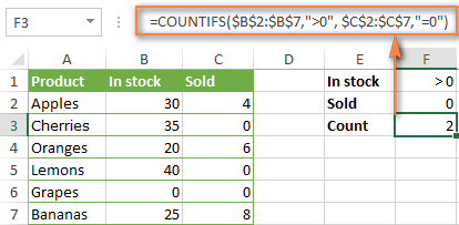
Suppose you have a product list like shown in the screenshot below. You want to get a count of items that are in stock (value in column B is greater than 0) but have not been sold yet (value is column C is equal to 0).
The task can be accomplished by using this formula:
=COUNTIFS(B2:B7,">0", C2:C7,"=0")
And the count is 2 ("Cherries" and "Lemons"):
Formula 2. COUNTIFS formula with two criteria
When you want to count items with identical criteria, you still need to supply each criteria_range / criteria pair individually.
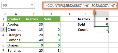
For example, here's the right formula to count items that have 0 both in column B and column C:
=COUNTIFS($B$2:$B$7,"=0", $C$2:$C$7,"=0")
This COUNTIFS formula returns 1 because only "Grapes" have "0" value in both columns.
Using a simpler formula with a single criteria_range like COUNTIFS(B2:C7,"=0") would yield a different result - the total count of cells in the range B2:C7 containing a zero (which is 4 in this example).
How to count cells with multiple criteria (OR logic)
As you have seen in the above examples, counting cells that meet all of the specified criteria is easy because the COUNTIFS function is designed to work this way.
But what if you want to count cells for which at least one of the specified conditions is TRUE, i.e. based on the OR logic? Overall, there are two ways to do this - by adding up several COUNTIF formulas or using a SUM COUNTIFS formula with an array constant.
Formula 1. Add up two or more COUNTIF or COUNITFS formulas
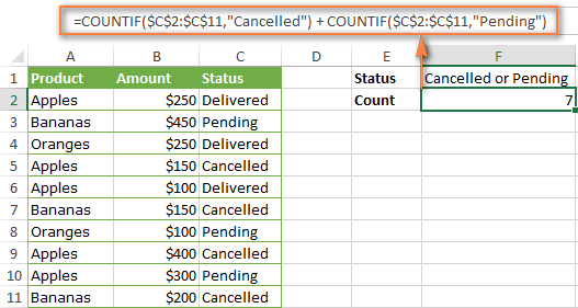
In the table below, supposing you want to count orders with the "Cancelled" and "Pending" status. To have it doen, you can simply write 2 regular Countif formulas and add up the results:
=COUNTIF($C$2:$C$11,"Cancelled") + COUNTIF($C$2:$C$11,"Pending")
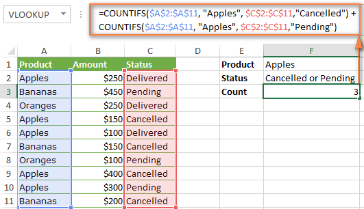
In case each of the functions is supposed to evaluate more than one condition, use COUNTIFS instead of COUNTIF. For example, to get the count of "Cancelled" and "Pending" orders for "Apples" use this formula:
=COUNTIFS($A$2:$A$11, "Apples", $C$2:$C$11,"Cancelled") + COUNTIFS($A$2:$A$11, "Apples", $C$2:$C$11,"Pending")
Formula 2. SUM COUNTIFS with an array constant
In situations when you have to evaluate a lot of criteria, the above approach is not the best way to go because your formula would grow too big in size. To perform the same calculations in a more compact formula, list all of your criteria in an array constant, and supply that array to the criteria argument of the COUNTIFS function. To get the total count, embed COUNTIFS inside the SUM function, like this:
In our sample table, to count orders with the status "Cancelled" or "Pending" or "In transit", the formula would go as follows:
=SUM(COUNTIFS($C$2:$C$11, {"cancelled", "pending", "in transit"}))
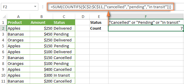
In a similar manner, you can count cells based on two or more criteria_range / criteria pairs. For instance, to get the number of "Apples" orders that are "Cancelled" or "Pending" or "In transit", use this formula:
=SUM(COUNTIFS($A$2:$A$11,"apples",$C$2:$C$11,{"cancelled","pending","in transit"}))

You can find a few more ways to count cells with OR logic in this tutorial: Excel COUNTIF and COUNTIFS with OR conditions.
How to count numbers between 2 specified numbers
By and large, COUNTIFS formulas for numbers fall into 2 categories - based on several conditions (explained in the above examples) and between the two values you specify. The latter can be accomplished in two ways - by using the COUNTIFS function or by subtracting one COUNTIF from another.
Formula 1. COUNTIFS to count cells between two numbers
To find out how many numbers between 5 and 10 (not including 5 and 10) are contained in cells C2 through C10, use this formula:
=COUNTIFS(C2:C10,">5", C2:C10,"<10")
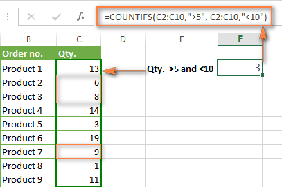
To include 5 and 10 in the count, use the "greater than or equal to" and "less than or equal to" operators:
=COUNTIFS(B2:B10,">=5", B2:B10,"<=10")
Formula 2. COUNTIF formulas to count numbers between X and Y
The same result can be achieved by subtracting one Countif formula from another. The first one counts how many numbers are greater than the lower bound value (5 in this example). The second formula returns the count of numbers that are greater than the upper bound value (10 in this case). The difference between the first and second number is the result you are looking for.
- =COUNTIF(C2:C10,">5")-COUNTIF(C2:C10,">=10") - counts how many numbers greater than 5 and less than 10 are in the range C2:C10. This formula will return the same count as shown in the screenshot above.
- =COUNTIF(C2:C10, ">=5")-COUNTIF(C2:C10, ">10") - the formula counts how many numbers between 5 and 10 are in the range C2:C10, including 5 and 10.
How to use cell references in COUNTIFS formulas
When using logical operators such as ">", "<", "<=" or ">=" together with cell references in your Excel COUNTIFS formulas, remember to enclose the operator in "double quotes" and
add an ampersand (&) before a cell reference to construct a text string.
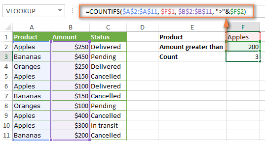
In a sample dataset below, let's count "Apples" orders with amount greater than $200. With criteria_range1 in cells A2:A11 and criteria_range2 in B2:B11, you can use this formula:
=COUNTIFS($A$2:$A$11, "Apples", $B$2:$B$11, ">200")
Or, you can input your criteria values in certain cells, say F1 and F2, and reference those cells in your formula:
=COUNTIFS($A$2:$A$11, $F$1, $B$2:$B$11, ">"&$F$2)
Please notice the use of absolute cell references both in the criteria and criteria_range arguments, which prevents the formula from being broken when copied to other cells.
For more information about the use of an ampersand in COUNTIF and COUNTIFS formulas, please see Excel COUNTIF - frequently asked questions.
How to use COUNTIFS with wildcard characters
In Excel COUNTIFS formulas, you can use the following wildcard characters:
- Question mark (?) - matches any single character, use it to count cells starting and/or ending with certain characters.
- Asterisk (*) - matches any sequence of characters, you use it to count cells containing a specified word or a character(s) as part of the cell's contents.
Tip. If you want to count cells with an actual question mark or asterisk, type a tilde (~) before an asterisk or question mark.
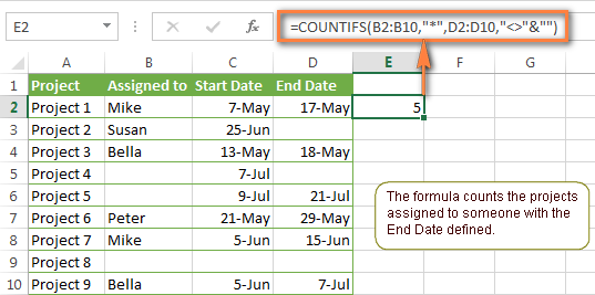
Now let's see how you can use a wildcard char in real-life COUNTIFS formulas in Excel. Suppose, you have a list of projects in column A. You wish to know how many projects are already assigned to someone, i.e. have any name in column B. And because we are learning how to use the COUNTIFS function with multiple criteria, let's add a second condition - the End Date in column D should also be set.
Here is the formula that works a treat:
=COUNTIFS(B2:B10,"*",D2:D10,"<>"&""))
Please note, you cannot use a wildcard character in the 2nd criteria because you have dates rather that text values in column D. That is why, you use the criteria that finds non-blank cells: "<>"&""
COUNTIFS and COUNTIF with multiple criteria for dates
The COUNTIFS and COUNTIF formulas you use for dates are very much similar to the above formulas for numbers.
Example 1. Count dates in a specific date range
To count the dates that fall in a certain date range, you can also use either a COUNTIFS formula with two criteria or a combination of two COUNTIF functions.
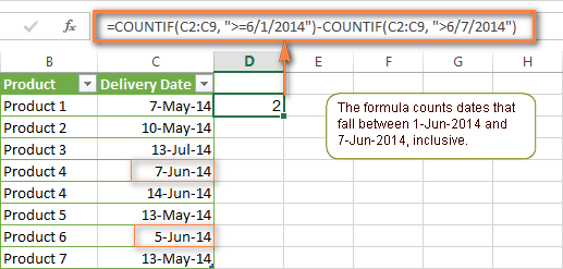
For example, the following formulas count the number of dates in cells C2 through C10 that fall between 1-Jun-2014 and 7-Jun-2014, inclusive:
=COUNTIFS(C2:C9, ">=6/1/2014", C2:C9, "<=6/7/2014")
=COUNTIF(C2:C9, ">=6/1/2014") - COUNTIF(C2:C9, ">6/7/2014")
Example 2. Count dates with multiple conditions
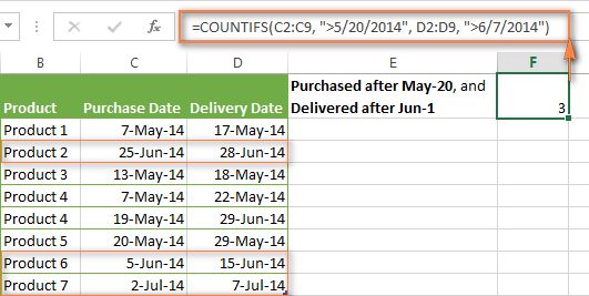
In the same manner, you can use a COUNTIFS formula to count the number of dates in different columns that meet 2 or more conditions. For instance, the below formula will find out how many products were purchased after the 20th of May and delivered after the 1st of June:
=COUNTIFS(C2:C9, ">5/1/2014", D2:D9, ">6/7/2014")
Example 3. Count dates with multiple conditions based on the current date
You can use Excel's TODAY() function in combination with COUNTIF to count dates based on the current date.
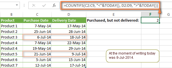
For example, the following COUNTIF formula with two ranges and two criteria will tell you how many products have already been purchased but not delivered yet.
=COUNTIFS(C2:C9, "<"&TODAY(), D2:D9, ">"&TODAY())
This formula allows for many possible variations. For instance, you can tweak it to count how many products were purchased more than a week ago and are not delivered yet:
=COUNTIFS(C2:C9, "<="&TODAY()-7, D2:D9, ">"&TODAY())
This is how you count cells with multiple criteria in Excel. I hope you will find these examples helpful. Anyway, I thank you for reading and hope to see you on our blog next week!
 by
by
1981 comments
Hi, I need a total count how often a student has achieved a grade of C or above (A*, A, B or C). The cells containing the grades are not next to each other so I need to have a range of data counted from separate cells and presented as one number.
Hello, Mark,
Please use this formula:
=CONCATENATE("A* = ",COUNTIF(A:A,"A*"),", A = ",COUNTIF(A:A,"A"),", B = ",COUNTIF(A:A,"B"),", C = ", COUNTIF(A:A,"C"))
Here A:A - is the range with the grades.
Hi I have a Excel Sheet, Where i have Numbers achieved by sales team like (In Column A)
1005,25900,5000,2005,1598,5368 etc..now i want to use a formula where i need to get the answer like..
if in Column a amount is upto 1000 then in column be it should count 2 points and if amount is in between 1001-2000 then 3, if amount is 2001-4000 then it should show as 5..
can u help on this
Hello, Charu,
Please enter the formula below to B1 and copy it across the column:
=IF(A1 < 1001, 2, IF(A1 < 2001, 3, IF(A1 < 4001, 5)))
How can I calculate the number of leads received during specific time ranges. E.g. how many leads did I received during 0:01:00 to 0:30:00 and so on.
I've 10,000s of leads received during 0:00:01 to 24:00:00. I am taking a time range of 30 minutes, 0:01 - 0:30, 0:31 - 1:00 an so on..
Hello, I have founded a very important function from this site.
thank you very much.
Count the number in Unic criteria. To say
I'm trying to use countif or countifs to count how many times a name shows up, the catch is there are many names, and I don't want to find all of them to do =countif(a5:a25,"JANE DOE"). Is there a way for excel to count and prompt the name & qty? I'm trying to calculate how many ECNs are assigned to individuals within a large group. Thank you for your help!
Hello, Jules,
Please try the following:
1. Select an empty cell in your table
2. Go to the Data tab -> Consolidate
3. Select Count from the Function drop-down list
4. Highlight the column with names and the one next to it
5. Tick the left column check-box and click OK.
Hope this helps.
my problem that conditional formatting in sheet formula that if date enter than red color how cell end count automatically red color
exp:-
09/01/2016
09/01/2016
how to count two cell red any formula
i have a table of employees by department and then a breakdown per day of holiday days and i need to count the amount of holiday days by department by month. is this possible?
Hello, Natasha,
For us to be able to help you better, please send us a sample table with your data in Excel. You can email it to support@ablebits.com. Please add the link to this article and your comment number.
Hello, I have been trying to figure out how to come up with a formula that counts cells from two different columns but that both represent one person. For example, I have an admitted column and a discharge column for clients. I'm looking at the first quarter of the fiscal year which counts October, November and December. However, when looking at each month individually, for example, October has clients that were admitted in August so I am trying to come up with something that counts before October but not after October as well as before November but not after November, etc. Does that make any sense? I apologize, I have been working on this for a while.
Hello, Mayra,
For us to be able to help you better, we need a sample table with your data in Excel. You can email it to support@ablebits.com. Please add the link to this article and your comment number.
A B
KPC164-FAB-Z13-BW20D-01#0001 19-Dec-15
KPC164-FAB-Z13-BW20D-01#0002 19-Dec-15
KPC164-FAB-Z14-BW20D-01#0002 15-Dec-15
KPC164-FAB-Z14-BW20D-01#0003 15-Dec-15
KPC164-FAB-Z15-BW20D-01#0023 05-Dec-15
KPC164-FAB-Z15-BW20D-01#0024 05-Dec-15
Hi!
I have 2 column in I need to count the date on column "B" with the corresponding text on column "A"
I want to count this : Z13-BW20D IF I HAVE CORRESPONDING DATE ON COLUMN "B"
Can some giving me a little help for this one?
Sample:
___________( column A)_____ (Colum B)
KPC164-FAB-Z13-BW20D-01#0001 19-Dec-15
KPC164-FAB-Z13-BW20D-01#0002 19-Dec-15
KPC164-FAB-Z14-BW20D-01#0002 15-Dec-15
KPC164-FAB-Z14-BW20D-01#0003 15-Dec-15
KPC164-FAB-Z15-BW20D-01#0023 05-Dec-15
KPC164-FAB-Z15-BW20D-01#0024 05-Dec-15
Please reply soon in my mail id.
Hi Svetlana Cheusheva Mam, Please solve my problem. There are subject codes and grades scattered in various columns & rows in excel sheet. How can i extract counted grades & codes in one cell of excel sheet jointly. What formula use in it. for example excel sheet given below yellow for your knowledge subject code 41 and next row grade A1 A2 B1 B2 C1 C2 D1 D2 .HOW TO COUNT TOTAL 41 A1 IS ............?
CANDIDATE NAME SUBJECT CODE MRK GRD SUBJECT CODE MRK GRD SUBJECT CODE MRK GRD SUBJECT CODE MRK GRD
RAM 30 99 A1 41 95 A1 30 99 A1 41 95 A1
SHYAM 41 99 A1 48 95 A1 41 99 A1 48 95 A1
RAJ 30 94 B1 41 88 A1 30 94 B1 41 88 A1
PHILP 37 92 A2 42 80 B1 37 92 A2 42 80 B1
PIKASO 41 80 A2 42 91 A1 41 80 A2 42 91 A1
PHAS 37 93 A1 42 81 B1 37 93 A1 42 81 B1
PARI 37 90 A2 42 70 B2 37 90 A2 42 70 B2
RAJ 30 88 A2 41 68 B2 30 88 A2 41 68 B2
RAMCHARAN 41 93 A1 42 82 A2 41 93 A1 42 82 A2
ANUPAM 41 77 B1 42 82 A2 41 77 B1 42 82 A2
VIJAY 41 80 A2 42 78 B1 41 80 A2 42 78 B1
VISHAL 41 82 A2 42 73 B2 41 82 A2 42 73 B2
VINAY 37 82 B1 42 65 C1 37 82 B1 42 65 C1
VIMAL 41 72 B1 42 67 C1 41 72 B1 42 67 C1
please give reply me as soon as possible.
CANDIDATE NAME SUBJECT CODE GRD SUBJECT CODE GRD SUBJECT CODE GRD SUBJECT CODE GRD
RAM 30 A1 41 A1 30 A1 41 A1
SHYAM 41 A1 48 A1 41 A1 48 A1
RAJ 30 B1 41 A1 30 B1 41 A1
PHILP 37 A2 42 B1 37 A2 42 B1
PIKASO 41 A2 42 A1 41 A2 42 A1
PHAS 37 A1 42 B1 37 A1 42 B1
PARI 37 A2 42 B2 37 A2 42 B2
RAJ 30 A2 41 B2 30 A2 41 E
RAMCHARAN 41 A1 42 A2 41 A1 42 A2
ANUPAM 41 B1 42 A2 41 B1 42 A2
VIJAY 41 A2 42 B1 41 A2 42 B1
VISHAL 41 A2 42 B2 41 A2 42 B2
VINAY 37 B1 42 C1 37 B1 42 C1
VIMAL 41 B1 42 C1 41 B1 42 C1
Sub. Code Total code A1 A2 B1 B2 C1 C2 D1 D2 E TOTAL
30 6 result here
41 20 8 6 4 1 0 0 0 0 1 20 IT IS MANUALLY COUNT AND WRITE
37 8
48 2
42 20
TOTAL IS MANUALY COUNT AND WRITE. YOU C A1 A2 B1 B2 C1 C2 D1 D2 & E BLOCK
I WANT FORMULA IN BLOCK THAT AUTOMATICALLY COUNT AND WRITE . I HELP YOU FOR YOUR UNDERSTANDING . ONE LINE
There are subject codes and grades scattered in various columns & rows in excel sheet.
How can I extract counted grades & codes in one cell of excel sheet jointly. for example code 41 get A1, A2 B1 B2 C1 C2 D1 D2 & E. for example given below.
Happy New Year Svetlana!
I would like to know how to find text in a range on a sheet that will display in a cell based on the criteria inputted in adjacent column:
So, I have an excel sheet "other sheet" showing a database of reg plates and vehicle type for a fleet of vehicles. On another sheet "current sheet", I need the vehicle type to display automatically in one column (see below where it says formula) when I type the reg plate number in the adjacent column.
THANKS :)
CURRENT SHEET OTHER SHEET
REG TYPE REG TYPE
A B 123 NISSAN
1 123 formula 321 LANDROVER
2 321 456 BUS
3 456
"CURRENT SHEET"
REG 123, 456, 345
TYPE FORMULA REQUIRED
"OTHER SHEET"
REG 123, 456, 345
TYPE NISSAN, LANDROVER, BUS
Hi Svetlana,
What formula can be used to find the count of cells that contain the text that is present in some other cell?
For eg. i can hardcord the formula like this: COUNTIF($E$3:$W$17,"Svetlana")
But instead of "Svetlana", i need to give the cell address.
*hardcode
Hi Mayur,
Nothing prevents you from supplying the cell address to the formula, e.g.:
=COUNTIF($E$3:$W$17,$A$1)
Hi Svetlana,
I'm trying to count the instances a value is less than zero given two dynamic column ranges match. They are named ranges 'universe' and 'markets'. I have the following formula to give me the total number of instances that I have a match but I'm not sure where to add the criteria to return how many of these matches are less than 0.
{=COUNT(IF(ISNUMBER(MATCH(universe,markets,0)),$A$7:$A$35))}
Thanks for having a look!
i have a data in excel sheet with cell content like this
the a 1,2,3
the p 1,2,3
how do i count the number of commas in the range with cell content.
i want the outcome like this
cell_contain count
"the a" 3
"the p" 3
i'll be very thankful if you provide answer for my query
How do I make a formula that states that column D is 30% of Column D?
Hi Sasha,
Probably there's some misprint here. Column D cannot be 30% of the same Column D :)
Hi Svetlana. Is it possible to use Countifs to pick up one of the criteria from a specific cell? I have tried, but it only ever returns a 0 value.
For example, I have a list of companies in column A, the month in which an order was delivered in column B, and a note of whether the goods were OK or faulty in column C. I want to find out how many orders were delivered faulty in a given month.
The formula
=COUNTIFS(B3:B100,"=03 (14/15)",C3:C100,"=Faulty")
works fine, but would it be possible to use another cell (let's say B102) to enter the month I am looking for and get Countifs to pick up and use the criteria from that cell?
Many thanks.
Hi David,
If my understanding it correct, you want a formula to "extract" a month number (03) from values in column B. If all the values in B have the same pattern like 03 (14/15), including a space before the opening parenthesis, you can use the following wildcard in criteria1:
=COUNTIFS(B3:B100, "03 (*", C3:C100,"=Faulty")
As for entering the month is a separate cell, probably it's also possible, but I cannot think of such a formula at the moment, sorry.
David,
Here's how you can count cells based on the month number in cell B102:
=COUNTIFS(B3:B100, B102&" (*",C3:C100,"Faulty")
Important! You should enter the month number in cell B102 exactly as it appears in column B (03 in your example). And since Excel cuts off leading zeros in numbers, 03 shall be entered in cell B102 as text (Home tab > Number group > Text).
Ok here is my question I have a multiple part number in one row and a serial number for each part number entered in a second row. I would like to count only the highest serial number for each of the different part numbers is this possible?
Trying to simplyfy the below functions:
C D
0 On Board
0A On Board
1A
3 On Board
=COUNTIFS(HK!C4:C8,"=0",HK!D4:D8,"=On Board")+COUNTIFS(HK!C4:C8,"=0A",HK!D4:D8,"=On Board")+COUNTIFS(HK!C4:C8,"=1",HK!D4:D8,"=On Board")+COUNTIFS(HK!C4:C8,"=1A",HK!D4:D8,"=On Board")
Tried this ... but no luck :(
=COUNTIFS(HK!C4:C8,{"=0","=0A","=1","=1A"},HK!D4:D8,"=On Board")
Need urgent help please..
Thanks
There's a File A and a File B, both in xls
Both have the two columns each of the same names, say, "1" and "2".
File A has 100 records. File B has 150 records.
We need to add a column "3" to File B, and put a value 'NotFound' in it if the value in "1" is not found anywhere in A's column "1".
After that is done, we need to repeat, in reverse. That is, add a column "3" to File A, and put a value "NotFound" in it if the value in A's "1" is not found anywhere in B's column "1".
Trying to create a count for check (Tick) marks (where "P" is a tick). I can have multiple ticks per box in Excel. Currently it wants to add each tick. If I add 1 more tick to a box (2 ticks in a box) it will subtract it instead of add on to my current total. How do I fix this?
My current syntax:
=COUNTIFS(C7:C25, "P", C7:C25, "P")
Please help. I need to be able to track my work.
Thanks.
my 1st column data is- =+COUNTIFS($G$5:$G$38,"ACTUAL",$H$5:$H$38,"D") this one
when i scroll it 2nd column the data is- =+COUNTIFS($G$5:$G$38,"ACTUAL",$H$5:$H$38,"D") this one
my question is why not data scrolled by column reference,where ever the data wants =+COUNTIFS($G$5:$G$38,"ACTUAL",$I$5:$I$38,"D")
plz chk and tell me the soluation
Thanks
CHUMAN
Dear All,
I need your help to show the total time spent between multiple two cells repeatedly.
For example, I'm starting my work by capturing the start time in A1 & ending at A2 and I'm getting the difference in A3 using the formula =A2-A1. After a short break, I'm again starting the time in A1 & ending in A2. Then what is the formula to be used to calculate the total timing spent in A4.
I have two columns, column 1- Dates, column 2- Names.
01/02/2015 ARYA
01/02/2015 ARYA
01/02/2015 ARYA
02/02/2015 ARYA
From the above example, I want the count to reflect 2, in other words I would want it to count as a single occurrence per day i.e., 01/02 - one occurrence & 02/02 one occurrence. Please help me with this. Please help me without date ranges as i need to use it for the entire year for different names.
when i scroll from one column to another column it have changes of his values
ie
=+COUNTIFS($G$5:$G$38,"ACTUAL",$H$5:$H$38,"D")
another one =+COUNTIFS($G$5:$G$38,"ACTUAL",$H$5:$H$38,"D") only copied where i want =+COUNTIFS($G$5:$G$38,"ACTUAL",$I$5:$I$38,"D")
Hi Svetlana,
If there are two columns A and B with following data:
A B
Apple 1
Banana 1
Orange 3
Apple 1
Apple 1
Banana 1
Banana 1
Banana 1
Banana 1
In the above data I would first like to search in column B for value 1 and then count only unique values in column A in such a manner that the function returns 2 (i.e., Apple and Banana). Is this possible and if so how can it be done?
I have data in Column F. The data is like either "M" or "MH", either "E" or "EH", either "N" or "NH". This is for counting Shifts.
I am using formula to count : =COUNTIFS(F4:F30,"=E",F4:F30,"=EH") for counting Evening Shifts. But it is givining me value as 0 (Zero). Please let me know where am I wrong.
Thanks for your help in advance.
I'm trying to get a total count of the values in one column, i.e. "Y100" and with all rows that contain that y100 count the number of cells in another column. i.e. "A". I've tried =COUNTIFS('Mods (Entire)'!B:B,"Y100",'Mods (Entire)'!C:C,"A") and =COUNTIFS('Mods (Entire)'!B:B,"=Y100",'Mods (Entire)'!C:C,"=A") both come back with a count of zero. Any and all help is greatly appreciated, will send sample if needed.
From the example above, if you use the following:
=COUNTIFS(B2:B11,"=0", C2:C11,"=0", D2:D11,"=0")
it will count from the row only if all three meet the criteria
however if you do:
=COUNTIFS(B2:B11,">0", C2:C11,">0", D2:D11,">0")
It will count from the row if any one, two, or all of the values is greater than 0
q1: how is that logical?
q2: How do I do the operation so that it counts only if all three satisfy the criteria
help on how to set COUNTIF to count only cell with >=25% but <=29% only,, meaning count only cells when it contains 25% and below 30%
I am trying to figure out a formal that would highlight a certain cell if a X appears a certain number of times within a certain data range. I am trying to work on an attendance sheet where i need the persons name to highlight if the attended 3 items in one data range and 2 in another data range and have data in another field that contains a drop drown list. I think i need to do a sum countif but I can't figure out how to set to highlight if a certain number within the data field is meet.
I want to count how many nonzero cells exists. All cells are time formatted. I am populating with elapsed time.
Column A - 0:00
Column B - 8:05
Column C - 9:22
I should get result as 2.
I am working with something like this:
COLUMN A COLUMN B COL.C COL.D
load# trailer# scac loc
uc856489 85694 SXTI y182
54852 SXTI y345
uc854585 95484 TAMI y652
45584524 6382 TAMI Y212
54585 SXTI Y121
UC845845 12548 JRWS Y222
I'm trying to find a rule that will let me see if there is get a count of empty trailers on the yard by scac code "SXTI" (COL C) BUT I don't want to calculate the loaded SXTI trailers (WHEN COLUMN A SHOWS A 3 STARTING WITH UC* OR 455) I was going to make a line for each scac code on a different sheet with the rule cell next to it just showing the number. Is there a way that will work for this? I have tried many combinations but can't seem to get it to work.
Hi,
Can you please help?
Example:
- M M N N
M V V D D
M V V V
N D V D E
N V E E
WE need do know how many "V" we have in the table with the conditions (Horizontal/Vertical) M/N ; M/N ; N/M ; N/M
The result is:
M/N = 1
M/M = 4
N/M = 2
N/M = 0
Many thanks in advance.
=COUNTIFS(C12>F12,">=1", C21>F21,">=1") ???
Basically looking to have a total for wins and losses in a sports results column.
So if 71 (C12) is greater than 70 (F12) give it a value of 1 (a win), then add that to the next line (C21) if that is a value of 1 as well.
I have 5 columns,
1. Date In
2. Time In
3. Date Out
4. Time Out
5. Date to count
I have a long list of these dates and times and want to find out by date and hour how many occurrences.
7a-8a
8a-9a
9-10a etc.
How do I assemble countifs to produce the hourly data?
Countifs(A1:A31,E1,B1:B31,">="&TIMEVALUE("7:00 AM"),B1:B31,="&TIMEVALUE("7:00 AM"),D1:D31,<="&TIMEVALUE"("8:00 AM")
I can't get to this to work so it shows between the in and out times and date.
Thank you,
Mike
HI,
I HAVE A EXCEL SHEET CONTAINS PERVIOUES HEALTH CHECK UP DATES AND I HAVE CREATED GRADES ACCORDIGNLY,
WANT TO FIX DATE FOR THE GRADES AS MENTION BELOW
IF GRADE A MEANS HAVE TO GET THE DATE OF NEXT HEALTH CHECK UP FROM PREVIOUS CHECK UPDATE WITH 180 DAYS ADDED
hi dear i dont have knowledg of excel formulas so plz guide me how learn a advance excel formula.
and i need your advice.
I would like to use a countif function in a pivot table. I have four columns of data with different suspension codes in each column. I might have violation "I01" appear in any of the four columns. I want to count how many times "I01" is in any of the four columns. I love the pivot table because then I can use them to count how many times this infraction is reported at each of the schools I work for. Any suggestions would be appreciated.
Hello,
This is my current formula for two different columns: =COUNTIF(B12:AF12,"lt") and =COUNTIF(B12:AF12,"d").
I am tracking Time, Attendance and other things for employees. If they have a late on one day (cell) I put LT and it counts it in the LT Column. If I put D for Disciplinary action it will count it on the D column but what if I have a late and Disciplinary action on the same day? I want it to count it on each different column and cell needed.
Thank you,
Eric
In Example 4. COUNTIF formulas with OR logic is there a reason you did not use the sum of the array?
=SUM(COUNTIFS(A2:A11,{"Product1","Product2}, B2:B11, 0))
I am also wondering the best way to count rows with multiple OR logic? I know the following doesn't work with 2 columns of OR logic, but what would be the best way to accomplish this?
=SUM(COUNTIFS(A2:A11,{"Product1","Product2}, B2:B11,{"0","14"}))
I've hit a brick wall with sheet that I am trying to Create to create a rota from a list of tasks that need to be performed at different times of the day. I have a list of tasks that must be performed and a person's name is input against it and the name is the automatically transferred to the rota by the formula.
I have set up the rota so that the cell under a specific time and persons name tests if the person has been allocated the task with the formula =IF(F8="Jane","task1","")
so that when Jane looks across the rota against her name she can see the tasks that have been allocated to her. This is working perfectly.
The problem is that at 12:00 Jane might be allocated any one of two tasks that need to be completed at the same time or no task at all. I have been trying to use the above formula and adding a second If statement onto it to test another cell if the first statement results in FALSE.
=IF(F8="Jane","task1",""),=IF(F10="Jane","task2","")
and this is not working.
Can you help?
Hi,
I need to simplify no of item for selected branch in a month? or to combine below countif formula.
1. TO COUNT NO OF ITEM IN JULY 2015
=COUNTIF(I:I,">=07/01/2015")-COUNTIF(I:I,">07/31/2015")
2. TO COUNT NO OF ITEM FOR BRANCH CODE "AG"
=COUNTIF(A:A,"=AG")
I want to compare two rowed cell values and find minimum between both,Minimum result number will be multiply by 3.5 and stored to third cell.
10
9
9*3.5
I'm trying to calculate how many times a state appears in a range. =COUNTIF('[2State Calendar.xlsx]Calendar'!$J$6:$K$11,"*NY*")
I want to calculate multiple states appearing in the same range. Is this possible?
Oh dear - that did not post correctly!
The first formula is =COUNTIFS($A$2:$A$10000,">=2420", $A$2:$A$10000,"="&$H2,$B$2:$B$10000,"<="&$I2) (where h2 and I2 are dates) and b is a column of dates
Hopefully that helps clarify.
Thanks,
Jo
Hi,
I need to count the number of postal codes within a certain range, e.g. between 2420 and 2490. I have been using the countifs function, however it does not seem to be counting all the postcodes that exist within the range specified (=COUNTIFS($A$2:$A$10000,">=2420", $A$2:$A$10000,"="&$H2,$B$2:$B$10000,"<="&$I2) - where h2 is a date and so is I2). I have also found that this formula is not counting all the dates that fall into this range in column b. Is there something also wrong with this formula?
I would appreciate any help I can get!
Thanks in advance,
Jo
True, Microsoft Excel 10 is the value of the F column. 6 When the value is put in the column H 4 value in column G to be put. I have required this type formula.