The tutorial explains how to use COUNTIFS and COUNTIF formulas with multiple criteria in Excel based on AND as well as OR logic. You will find a number of examples for different data types - numbers, dates, text, wildcard characters, non-blank cells and more.
Of all Excel functions, COUNTIFS and COUNTIF are probably most often mixed up because they look very much alike and both are purposed for counting cells based on the specified criteria.
The difference is that COUNTIF is designed for counting cells with a single condition in one range, whereas COUNTIFS can evaluate different criteria in the same or in different ranges. The aim of this tutorial is to demonstrate different approaches and help you choose the most efficient formula for each particular task.
Excel COUNTIFS function - syntax and usage
The Excel COUNTIFS function counts cells across multiple ranges based on one or several conditions. The function is available in Excel 365, 2021, 2019, 2016, 2013, Excel 2010, and Excel 2007, so you can use the below examples in any Excel version.
COUNTIFS syntax
The syntax of the COUNTIFS function is as follows:
- criteria_range1 (required) - defines the first range to which the first condition (criteria1) shall be applied.
- criteria1 (required) - sets the condition in the form of a number, cell reference, text string, expression or another Excel function. The criteria defines which cells shall be counted and can be expressed as 10, "<=32", A6, "sweets".
- [criteria_range2, criteria2]… (optional) - these are additional ranges and their associated criteria. You can specify up to 127 range/criteria pairs in your formulas.
In fact, you don't have to remember the syntax of the COUNTIF function by heart. Microsoft Excel will display the function's arguments as soon as you start typing; the argument you are entering at the moment is highlighted in bold.

Excel COUNTIFS - things to remember!
- You can use the COUNTIFS function in Excel to count cells in a single range with a single condition as well as in multiple ranges with multiple conditions. If the latter, only those cells that meet all of the specified conditions are counted.
- Each additional range must have the same number of rows and columns as the first range (criteria_range1 argument).
- Both contiguous and non-contiguous ranges are allowed.
- If the criteria is a reference to an empty cell, the COUNTIFS function treats it as a zero value (0).
- You can use the wildcard characters in criteria - asterisk (*) and question mark (?). See this example for full details.
How to use COUNTIFS and COUNTIF with multiple criteria in Excel
Below you will find a number of formula examples that demonstrate how to use the COUNTIFS and COUNTIF functions in Excel to evaluate multiple conditions.
How to count cells with multiple criteria (AND logic)
This scenario is the easiest one, since the COUNTIFS function in Excel is designed to count only those cells for which all of the specified conditions are TRUE. We call it the AND logic, because Excel's AND function works this way.
Formula 1. COUNTIFS formula with multiple criteria
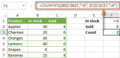
Suppose you have a product list like shown in the screenshot below. You want to get a count of items that are in stock (value in column B is greater than 0) but have not been sold yet (value is column C is equal to 0).
The task can be accomplished by using this formula:
=COUNTIFS(B2:B7,">0", C2:C7,"=0")
And the count is 2 ("Cherries" and "Lemons"):
Formula 2. COUNTIFS formula with two criteria
When you want to count items with identical criteria, you still need to supply each criteria_range / criteria pair individually.
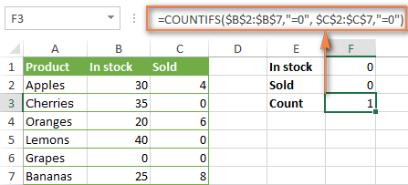
For example, here's the right formula to count items that have 0 both in column B and column C:
=COUNTIFS($B$2:$B$7,"=0", $C$2:$C$7,"=0")
This COUNTIFS formula returns 1 because only "Grapes" have "0" value in both columns.
Using a simpler formula with a single criteria_range like COUNTIFS(B2:C7,"=0") would yield a different result - the total count of cells in the range B2:C7 containing a zero (which is 4 in this example).
How to count cells with multiple criteria (OR logic)
As you have seen in the above examples, counting cells that meet all of the specified criteria is easy because the COUNTIFS function is designed to work this way.
But what if you want to count cells for which at least one of the specified conditions is TRUE, i.e. based on the OR logic? Overall, there are two ways to do this - by adding up several COUNTIF formulas or using a SUM COUNTIFS formula with an array constant.
Formula 1. Add up two or more COUNTIF or COUNITFS formulas
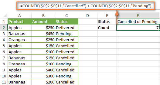
In the table below, supposing you want to count orders with the "Cancelled" and "Pending" status. To have it doen, you can simply write 2 regular Countif formulas and add up the results:
=COUNTIF($C$2:$C$11,"Cancelled") + COUNTIF($C$2:$C$11,"Pending")
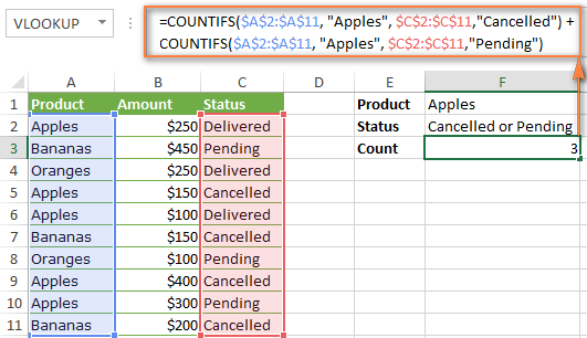
In case each of the functions is supposed to evaluate more than one condition, use COUNTIFS instead of COUNTIF. For example, to get the count of "Cancelled" and "Pending" orders for "Apples" use this formula:
=COUNTIFS($A$2:$A$11, "Apples", $C$2:$C$11,"Cancelled") + COUNTIFS($A$2:$A$11, "Apples", $C$2:$C$11,"Pending")
Formula 2. SUM COUNTIFS with an array constant
In situations when you have to evaluate a lot of criteria, the above approach is not the best way to go because your formula would grow too big in size. To perform the same calculations in a more compact formula, list all of your criteria in an array constant, and supply that array to the criteria argument of the COUNTIFS function. To get the total count, embed COUNTIFS inside the SUM function, like this:
In our sample table, to count orders with the status "Cancelled" or "Pending" or "In transit", the formula would go as follows:
=SUM(COUNTIFS($C$2:$C$11, {"cancelled", "pending", "in transit"}))
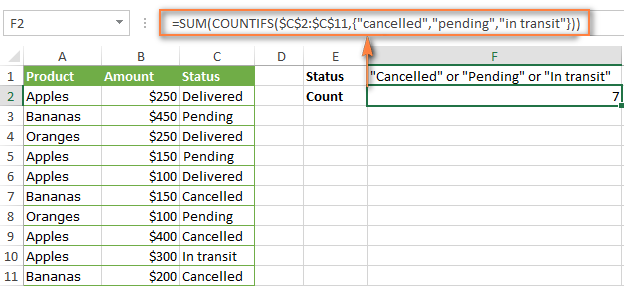
In a similar manner, you can count cells based on two or more criteria_range / criteria pairs. For instance, to get the number of "Apples" orders that are "Cancelled" or "Pending" or "In transit", use this formula:
=SUM(COUNTIFS($A$2:$A$11,"apples",$C$2:$C$11,{"cancelled","pending","in transit"}))

You can find a few more ways to count cells with OR logic in this tutorial: Excel COUNTIF and COUNTIFS with OR conditions.
How to count numbers between 2 specified numbers
By and large, COUNTIFS formulas for numbers fall into 2 categories - based on several conditions (explained in the above examples) and between the two values you specify. The latter can be accomplished in two ways - by using the COUNTIFS function or by subtracting one COUNTIF from another.
Formula 1. COUNTIFS to count cells between two numbers
To find out how many numbers between 5 and 10 (not including 5 and 10) are contained in cells C2 through C10, use this formula:
=COUNTIFS(C2:C10,">5", C2:C10,"<10")
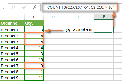
To include 5 and 10 in the count, use the "greater than or equal to" and "less than or equal to" operators:
=COUNTIFS(B2:B10,">=5", B2:B10,"<=10")
Formula 2. COUNTIF formulas to count numbers between X and Y
The same result can be achieved by subtracting one Countif formula from another. The first one counts how many numbers are greater than the lower bound value (5 in this example). The second formula returns the count of numbers that are greater than the upper bound value (10 in this case). The difference between the first and second number is the result you are looking for.
- =COUNTIF(C2:C10,">5")-COUNTIF(C2:C10,">=10") - counts how many numbers greater than 5 and less than 10 are in the range C2:C10. This formula will return the same count as shown in the screenshot above.
- =COUNTIF(C2:C10, ">=5")-COUNTIF(C2:C10, ">10") - the formula counts how many numbers between 5 and 10 are in the range C2:C10, including 5 and 10.
How to use cell references in COUNTIFS formulas
When using logical operators such as ">", "<", "<=" or ">=" together with cell references in your Excel COUNTIFS formulas, remember to enclose the operator in "double quotes" and
add an ampersand (&) before a cell reference to construct a text string.
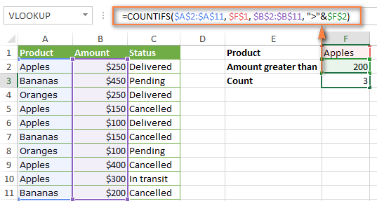
In a sample dataset below, let's count "Apples" orders with amount greater than $200. With criteria_range1 in cells A2:A11 and criteria_range2 in B2:B11, you can use this formula:
=COUNTIFS($A$2:$A$11, "Apples", $B$2:$B$11, ">200")
Or, you can input your criteria values in certain cells, say F1 and F2, and reference those cells in your formula:
=COUNTIFS($A$2:$A$11, $F$1, $B$2:$B$11, ">"&$F$2)
Please notice the use of absolute cell references both in the criteria and criteria_range arguments, which prevents the formula from being broken when copied to other cells.
For more information about the use of an ampersand in COUNTIF and COUNTIFS formulas, please see Excel COUNTIF - frequently asked questions.
How to use COUNTIFS with wildcard characters
In Excel COUNTIFS formulas, you can use the following wildcard characters:
- Question mark (?) - matches any single character, use it to count cells starting and/or ending with certain characters.
- Asterisk (*) - matches any sequence of characters, you use it to count cells containing a specified word or a character(s) as part of the cell's contents.
Tip. If you want to count cells with an actual question mark or asterisk, type a tilde (~) before an asterisk or question mark.
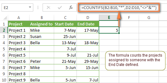
Now let's see how you can use a wildcard char in real-life COUNTIFS formulas in Excel. Suppose, you have a list of projects in column A. You wish to know how many projects are already assigned to someone, i.e. have any name in column B. And because we are learning how to use the COUNTIFS function with multiple criteria, let's add a second condition - the End Date in column D should also be set.
Here is the formula that works a treat:
=COUNTIFS(B2:B10,"*",D2:D10,"<>"&""))
Please note, you cannot use a wildcard character in the 2nd criteria because you have dates rather that text values in column D. That is why, you use the criteria that finds non-blank cells: "<>"&""
COUNTIFS and COUNTIF with multiple criteria for dates
The COUNTIFS and COUNTIF formulas you use for dates are very much similar to the above formulas for numbers.
Example 1. Count dates in a specific date range
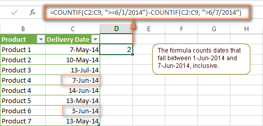
To count the dates that fall in a certain date range, you can also use either a COUNTIFS formula with two criteria or a combination of two COUNTIF functions.
For example, the following formulas count the number of dates in cells C2 through C10 that fall between 1-Jun-2014 and 7-Jun-2014, inclusive:
=COUNTIFS(C2:C9, ">=6/1/2014", C2:C9, "<=6/7/2014")
=COUNTIF(C2:C9, ">=6/1/2014") - COUNTIF(C2:C9, ">6/7/2014")
Example 2. Count dates with multiple conditions
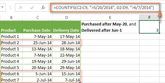
In the same manner, you can use a COUNTIFS formula to count the number of dates in different columns that meet 2 or more conditions. For instance, the below formula will find out how many products were purchased after the 20th of May and delivered after the 1st of June:
=COUNTIFS(C2:C9, ">5/1/2014", D2:D9, ">6/7/2014")
Example 3. Count dates with multiple conditions based on the current date
You can use Excel's TODAY() function in combination with COUNTIF to count dates based on the current date.
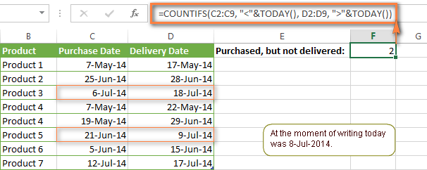
For example, the following COUNTIF formula with two ranges and two criteria will tell you how many products have already been purchased but not delivered yet.
=COUNTIFS(C2:C9, "<"&TODAY(), D2:D9, ">"&TODAY())
This formula allows for many possible variations. For instance, you can tweak it to count how many products were purchased more than a week ago and are not delivered yet:
=COUNTIFS(C2:C9, "<="&TODAY()-7, D2:D9, ">"&TODAY())
This is how you count cells with multiple criteria in Excel. I hope you will find these examples helpful. Anyway, I thank you for reading and hope to see you on our blog next week!
 by
by
1979 comments
Dear Svetlana,
Greetings, we meet again. I was trying to put a formula by using COUNTIFS, but it is coming with Error that too many arguments. Can you please advise.
A B C
Details Payment Authority to Waive
Bill 5000 If the value in B2 is less than 5000 then
Manager, more than 5000 than General Manager,
more than 10000 it will be Director.
Late Fine 6000 The value will show Manager
Dear Svetlana,
Greetings, we meet again. I was trying to put a formula by using COUNTIFS, but it is coming with Error that too many arguments. Can you please advise.
A B
Details Payment Authority to Waive
Payment 5000 If the value in B2 is less than 5000 then Manager, more than 5000 than General Manager, more than 10000 it will be Director
Late Payment If the value in B3 is less than 5000 then Manager, more than 5000 than General Manager, more than 10000 it will be Director
Cancellation Fee If the value in B4 is less than 5000 then Manager, more than 5000 than General Manager, more than 10000 it will be Director
Total Waiver If the value in B5 is less than 5000 then Manager, more than 5000 than General Manager, more than 10000 it will be Director
Total Liability If the value in B6 is less than 5000 then Manager, more than 5000 than General Manager, more than 10000 it will be Director
Hi,
I need to count total numbers >4 for Keith from 1st to 3rd June.
Countifs only counts one column (EG: 1st June). what formula can i use to count from all 3 column.
June 1 June 2 June 3
Keith 9 4 8
Keith 8 5 2
Keith 5 2 7
Ryan 6 1 9
Keith 2 3 5
Ryan 5 6 4
Keith 4 5 3
Ryan 5 8 2
Hi,
I am currently using the formula =IF(U2+V2<TODAY(),"X","OK") but want to include and or Q2 is Y = "OK" or N = "X"
How can i write this?
Hi,
I am currently using the formula =IF(U2+V2<TODAY(),"X","OK") but want to include and or Q2
Hello,
i have 1754 cells , with each cell contains 5 different numbers ranging from 01 to 31.
now i want frequency of each individual number from 01 to 31.,for all this 1754 cells.,
what should i do?.,
How to sum all wins (sheet one B3:B16 ) from sheet one on a specific date (sheet one A3:A16) and then sum this in sheet two's cell F3 "IF" F3 is the same date as in E3 date/timestamp?
Link to example sheet : https://docs.google.com/spreadsheets/d/18kt1RM2OrNmeAGWfphXwZFFyJ4Zwk_d-QibwnNPLaPg/edit#gid=1901723577&range=A1:H16
In this example i would like (sheet two to be filled like this)
F3 is = 3 and G3 = 2 and H3 = 2
F4 is = 1 G4 = 1 and H4 = 1
F5 is = blank G5 = 1 H5 = 1
F6 is = blank G6 = blank H5 = blank
F7 is = 1 G7 = blank H7 = blank
F8 is = blank G8 = blank H8 = 1
Any help appreciated :)
Regards Ronni
Hello, Ronny,
use the following COUNTIFS function:
for F3: =COUNTIFS(Sheet1!B1:B14,"Win",Sheet1!A1:A14,Sheet1!A1)
With its help we're looking for "Win" in the second column of Sheet1 if its first column contains the date from A1. The same goes for losses and ties:
for G3: =COUNTIFS(Sheet1!B1:B14,"Otm",Sheet1!A1:A14,Sheet1!A1)
for H3: =COUNTIFS(Sheet1!B1:B14,"Tie",Sheet1!A1:A14,Sheet1!A1)
To count the values under the other dates, simply change the cell reference at the end of the formula:
for F4: =COUNTIFS(Sheet1!B1:B14,"Win",Sheet1!A1:A14,Sheet1!A10)
Do hope this solves your task!
i want to make summary for the monthe in date wise
Dear i need one help
how do i count the data for each date
Actual Date Too early Ontime Delay
01/06/17 01/06/17
01/06/17 02/06/17
01/06/17 03/06/17
01/06/17 04/06/17
01/06/17 05/06/17
01/06/17 06/06/17
01/06/17 07/06/17
01/06/17 08/06/17
01/06/17 09/06/17
01/06/17 10/06/17
02/06/17 11/06/17
05/06/17 12/06/17
06/06/17 13/06/17
Hi Svetlana
In my Workbook, there is multiple sheet with data.
Just for Example,
I have a multiple sheet's which name is Jan, Feb, Mar, Apr, May, jun etc.
In final sheet I have 1 data validation cell (R11) with Name like, Kinjal, Mittal, Shankar, Nirav, etc.
and In Final Sheet I used one formula like: =COUNTIF(Jan!A7:N100,R11)*100/P9
Where "Jan" is a Sheet name, "A7:N100" is a index, R11 is a data validation shall with multiple name, and P9 is a constant value.
My problem is that, I want to used Data validation cell with multiple sheet name. So I want in final sheet two data validation cell and one cell for formula.
For Example: if K8 is data validation cell with data of Jan, Feb, Mar, Apr, May, jun etc.
and
R11 is another data validation cell with data of Kinjal, Mittal, Shankar, Nirav, etc.
So which formula I can used instead of below
Jan!A7:N100,R11)*100/P9
I don't want to used name of sheet, I want to used data validation cell for sheet name.
Hello,
please I need you help here
actors roles action_date
Milan B approver
Milan C reviewer 15/01/2017
Milan B reviewer
Milan B reviewer 13/05/2017
Milan C reviewer 13/05/2017
Milan B approver 13/05/2017
Milan B reviewer 13/05/2017
Milan C reviewer 13/05/2017
Milan B approver 13/05/2017
Milan C reviewer 13/05/2017
Milan B approver 13/05/2017
Milan C reviewer 13/05/2017
I want to wrire a count formula which can give me how many time MIlan B was reviewer in Date 13/05/2017
Merci
Column A data like 1, 2, 4, 3, 5, 8, 10.
COlumn B data like 8, 10, 12, 8, 6 ,12, 15
can i use sumifs/ counifs, making sure to give value a score of 2 if it is more than 2 in column a, and score of 0, if it is less than 2, and score of 1 if it is equals to 2.
For column B, it is same scoring except for value is 10 instead of 2.
and them sum up them
Many thanks for this, after finding this post I had the formulas I needed done in 5 minutes!
Svetlana,
Thanks for the post - I needed something to count multiple criteria over two columns. Your formula with the arrays worked flawlessly and is exactly what I needed!
Thanks
Troy
Hi,
Have a problem here too.
Monday Tuesday
12:30 06:00
06:30
06:30
06:30
12:30
12:30
06:30
For example we only got 3 staffs to work at 06:30, but above you will see that there were 4 or maybe more rostered. I want to know
Hi,
Have a problem here too.
Monday Tuesday
12:30 06:00
06:30 06:30
06:30 06:30
06:30 06:30
12:30 06:30
12:30 12:30
06:30 12:30
For example we only got 3 staffs to work at 06:30, but above you will see that there were 4 or maybe more rostered. if the count of 06:30 is exceeded to 3, then I want to put "Exceeded" or maybe "06:30 Exceeded"
Hi Team
Please can I have your help with the following query.
I have a spreadsheet with 4 columns, A: item being made, B: value, C: date I want it completed and D: blank or date completed.
From this information I want to extract the following:
Completed on time
Completed Late
Running Late
On track
Any help with the formula for these would be hugely appreciated - Thank you!
Hi Svetlana,
I have a query but for that I have for upload data because I not able to explain without data. Is it possible to share data with you?
Hi Svetlana,
I need your help with following query.
I have a table where Column A is with multiple date values (LAST DATE OF SUBMISSION) and Column B is with multiple date values (DATE SUBMITTED). now my query is to count number of cells where date of submission is lower or equal to last date of submission. Each row may have different "LAST DATE OF SUBMISSION" OR "DATE SUBMITTED".
The formula should return a value which represents how many quotations have been submitted before the deadline in a range and omit those which are submitted after the deadline.
Hi Brittany,
I have an Attendance sheet in which i use code like CL(casual leave) H(Half day) the problem is that i want to do a horizontal calculation in such a way tht i get an employee attendance total like if there is CL for four days it should add 1 for every CL and add 0.5 for every H.
Please help me i will really appreciate
Hello team, I need your help.
I'm working on a Daily Personnel Time sheet, where on rows I have the list of all projects, and they can be repeated due to different activities. And on the columns I have the list of people, positions, nationality. There we put the hours spent by each person for each particular activity. So the question is I want to count positions involved for each project, I used sumproduct but was not successful since it gives me the sum of the hours spent, then I used formula "IF" on the hours substituting the hours greater than 0 into 1. But this is still not working since the formula counted a person who was involved in the same project but in different activities. Could you help me please,
Thank you in advance,
Best Regards,
Miras
=((COUNTIFS(April!B4,"yes", April!G4,"yes", April!J4:S4, "*")))
How come this isn't working?
This works
=((COUNTIFS(April!B4,"yes", April!G4,"yes", April!J4, "*")))
The astrick just means at least one of the cells is not blank.
I need the cells that are considered to be j4 through s4 not just one of them...
Please help!
I am sorry I spelled asterisk wrong... My head hurts haha
Hi Brittany,
The point is that the COUNTIFS syntax requires each additional range be the same size as the first range, i.e. have the same number of rows and columns. Therefore, you cannot supply one cell to the criteria_range1 argument and a range of cells to a subsequent criteria range. So, I am afraid you will have to list every cell j4 through s4 individually in your formula.
That would mean every cell in that range would have to be filled in order for it to be counted as one. I just need at least one of the cells filled. Is there a way to do that?
Brittany,
You can use one of the following formulas as a working alternative to your first formula:
=IF(AND(G4="yes",B4="yes",COUNTIF(J4:S4,"*")>0),1,0)
=--(B4="yes")*(G4="yes")*(COUNTIF(J4:S4,"*")>0)
The formulas return 1 if B4 is "yes", G4 is "yes" and at least one cell in the range J4:S4 contains any text (please note, "*" counts only text values, but does not count numbers); 0 otherwise.
However, I am not sure I understand your ultimate goal correctly. If you want to achieve something different, please clarify.
I need to find the MAX number in a range with conditions. As in cell value
equals =MAX(COUNTIFS(Sheet1!$I$2:$I$999,"Yes",Sheet1!$U$2:$U$999,"NNN")L2:L999)
Where L2:L999 is the range that I need the maximum returned.
I have tried a few combinations, but unable to work it out.
Your formula won't work (by the way, it misses comma after the first parameter).
You need to use MAXIFS function (but it works in Excel 2016 only):
=MAXIFS(L2:L999, Sheet1!$I$2:$I$999,"Yes",Sheet1!$U$2:$U$999,"NNN")
You can read more about MAXIFS here.
For other Excel versions use array formula (entered by Ctrl+Shift+Enter):
=MAX((Sheet1!$I$2:$I$999="Yes")*(Sheet1!$U$2:$U$999="NNN")*L2:L999)
Thanks Natalia.
Unfortunately the array (Ctrl+Shift+Enter) didn't work either. (example below)
=MAX((Sheet1!I2:I999="Yes")*(Sheet1!U2:U999="NNN")*Sheet1!L2:L999)
Recap: I need to return the maximum figure (Column L) the meets certain parameters I = Yes and U = NNN. I have tried this certain ways but have not had any success.
Any help would be greatly appreciated.
I got it to work with this.
{=MAX(IF((Sheet1!$I$2:$I$999="yes")*(Sheet1!$G$2:$G$999="NAT"),(Sheet1!$L$2:$L$999)))}
Thank you.
Can you help me pls?
Example
Roll No. | I | II |
-------------------
1 04 05
2 11 12
3 05 04
4 10 04
How to count Coloum minimum or maximum total in excel
Hello Team, I'm struggling with the countifs function, I am trying to count data in a range of columns, in one column "A" I have a list of dates ranging from 1996 to 2017, in columns "B","C","D" etc. I have other data mostly Numbers. What I would like to accomplish is as follows
If its Jan 1 I would like all the years (21 years on Jan 1) Of the specially data I choose in cell H6. Is this task possible? Any help would be much appreciated.
I only want to include Apples and Oranges from Col A that were also sold after 1/1/2015 and before 1/1/2016 (Col C) and are both currently paid for OR on a tab (Col D). Its the currently paid for OR on a tab where I am failing. There are no Apples and Oranges that are both paid for and also on a tab. I want all the oranges and apples that are either paid for or on a tab...So far I've got: =COUNTIFS($A$1:$A$599,"Apples",$A$1:$A$599,"Oranges",$C$1:$C$599,">=1/1/2015",$C$1:$C$599,"<1/1/2016",$D$1:$D$599,"Current",OR,"Tab")
Getting a $NAME? result. I can run just the dates and it works. I can run just looking for apples and oranges...I can get it to give me separately the paid and on tab correctly.
Hey, Cher,
your formula should look like this:
=SUM(COUNTIFS($A$1:$A$599,{"Apples","Oranges"},$A$1:$A$599,$C$1:$C$599,">=1/1/2015",$C$1:$C$599,"<1/1/2016",$D$1:$D$599,"Current")+SUM(COUNTIFS($A$1:$A$599,{"Apples","Oranges"},$A$1:$A$599,$C$1:$C$599,">=1/1/2015",$C$1:$C$599,"<1/1/2016",$D$1:$D$599,"Tab")
It can be written as an array formula, but it would be too difficult to understand. Read this topic for more details.
Suppose i have a list of marks as follows:
A B
1. 11
2. 4
3. 1
4. 12
5. 4
6. 7
7. 9
8. 12
9. 3
10. 20
Then use th countifs fontion to obtain thé first mark range ex. Countifs(B1:B11,>=O,B1:B11,<5) to obtain thé number of marks ranging from 0-4, what can I do to automatically produce the counts of the other ranges, say 5to<7, 7to<9, 9to<10, 10to<12, 12to<14, 14to<20
Thanks in advance
Heya! I am having a hard time getting a formula to work that counts a Y in one of 3 columns to the right if a rep's initials are in the column to the left. So I've tried:
=SUM(COUNTIFS(A3:A1002,{"JM"})+COUNTIFS(G3:G1002,{"Y"},I3:I1002,{"Y"},K3:K1002,{"Y"}))
=COUNTIFS(A3:A1002,"JH", G3:G1002,"Y", I3:I1002,"Y", K3:K1002,"Y")
I can get it to work with one, but not all 3 columns (which are for 3 sessions in one day).
Hello, Cher,
try this one:
=SUM(IF((--($A$3:$A$1002="JH"))*((G3:G1002="Y")+(I3:I1002="Y")+(K3:K1002="Y"))>0,1,0))
Note, that this should be an array formula and you need to press Ctrl + Shift + Enter instead of Enter.
The formula adds 1 whenever there's 'JH' in column A AND any of G,I,K columns contain 'Y'.
Hope it helps.
Dear Sir/ Madam
I am having the Two sheet One Sheet Containing the Results & another Sheet Containing Numbers. if I am giving the formula of
Result Sheet Containing : Number of 4 digits 9923, 0120, 0140, 0150, 0170
Coupon Number Containing
From NO: 10009882 To :10010763. i have to take Only Last 4 Digits that should be match in Result Sheet. Formula is given below.
COUNTIFS(Result!$B$3:$B$102,">="&RIGHT(J67,4),Result!$B$3:$B$102,"<="&RIGHT(K67,4)))*10
Coupon Amount is coming 0. Please give the Solution
I previously submitted a question on tallying X's in random cells and gave a display of what I had input. I realized that I hadn't continue to put COuNTIF however, even once I did, I was still getting an error. The cells are not contiguous and contain an x. I am trying to find a way of tallying individual cells across a row that are not within a range.
Any help is appreciated.
Hi...I am a trying use Countifs with multiple criteria for dates, but am having difficulty. Here's the scenario:
C3=07/01/16 - Format is Date
D3=07/31/16 - Format is Date
Formula:
=COUNTIFS(Assigned,$A6,OpenedAt,">=&C3", OpenedAt, "=&C3" I get a total, but when I add the second criteria, it calculates to zero...and yes there are items that are greater than 07/01/16.
Thanks for any help you can give.
I have three columns that I need to sort data on but I just cant get it right.
I need to count the number of occurrence's if it meets criteria in three different columns.
Thanks so much,
I have different numbers spread across rows and columns. The numbers have different values, of which some are unique and some reoccurring. I need the numbers and the count(occurance) of each numbers.
Can you help me please.
Good Morning,
I am trying to create a formula that will count all of the "1"'s in a particular column but some of the cells have more than one number separated by commas. I have attempted to count this data using the formula: =COUNTIF('Part 1 Imput'!A7:A700,"*1*")+('Part 1 Imput'!A7:A700,"1"). I unfortunately am getting an error. Can you please help me find my error or am I thinking about this wrong?
Thank you
Hi,
Please could you let me know how I could make the following formula work:
=COUNTIFS('Raw Data'!C:C,"="&Summary!$D$4,'Raw Data'!E:E,""&Summary!B10,'Raw Data'!H:H,"")
I think the last criteria is overwriting the third criteria so I just get 0. Is there a way that I can add an OR statement into the formula?
Many Thanks
I have a list of Call Agents and the times that they logged into their phone and log out of their phone, and I would like to create a listing of how many Call Agents are staffed by the half hour from 08:00 to 20:00
What I have
(10 Agents)
Log in - E2=09:27
Log out - F2 = 16:00
Agent 2 E3 and F3
Agent 3 E4 and F4
What I want
08:00 - 08:30 X number agents available
08:30 - 09:00 X number of agents available
""
""
""
19:30 - 20:00 X number of agents available
Dear,
Could you please send me e-mail, i really need your help.
Thank you.
Best regards,
Nermana Čubro
Amazing. COUNTIFS was exactly what I was looking for. Worked perfect and pretty straight forward function to use.
Thanks a lot!!
I want to first check to see if certain text exists in a cell, if it does exist, then I want to do a calculation on 2 other cells.Right now I'm checking for the ext and assigning that a value of 1 in one cell, then in another cell (example cell a3 now =1), if the 1 exists then calculation a5-a4 (example)
Hi,
I'm trying to create a formula which predicts a date in the future. If column A has the 'F' in the date will be 30 days in the future, if it has 'D' then 90 days, if 'E' then 180 days. However I want it to be calculated from the last date entered in four cells. example
A=F B=01/01/17 C=02/02/17 d=02/03/17 E='Blank' F=30 days from D
or A=E B=01/01/17 C=02/02/17 d='Blank' E='Blank' F=180 days from C
Hi
Im trying to create a formula to lookup if all cells between a date range all equal "Yes" I have the formula below to count the cells between the date ranges just wondering how to modify this to see if all cells contain "Yes"
=SUMIFS($B6:$BA6,$B$5:$BA$5,">="&$BE$3,$B$5:$BA$5,"<="&$BE$4)
I am looking for a formula to help with headcounts on days of the week and between certain times.
I have 2 columns, one for days of the week and one for the time visited. I am looking to gather the information in a chart at the end of each month/qtr to look for the visit trends.
Example:
Mon 6pm
Mon 1145am
Tue 1pm
Wed 9am
Wed 8pm
Thu 945am
Thu 1215pm
Fri 10am
Sat 236pm
Sat 1130pm
Sun 4pm
Sun 6pm
And so on for a month. I need a count of all the Mon visits between 10a-1259pm, 1pm-359pm,4p-659pm, 7pm-959pm,10p-1259am and 1am-559am.
Any help would be appreciated!
hello, admin I've been following your tutorials since a month now could you help me on my problem please?, I want to count the number of minutes late of our employees, our official time is 7:00:00 AM, but i am looking everywhere for this formula but I couldn't find anywhere until I found this article of yours. I Think this is related on my problem.
Advance,
J.V.
Send me a sample please.
remindfwd[at]gmail[dot]com
replace "[AT]" and "[DOT]" with respective signs.
Perhaps you can use TIMEVALUE formula, but you haven't share any info in the comment.
Regards!
You can enter into cell D2 the value 7:00:00 AM.
In column A you have names
In column B times arivee :)
Your "table" have headers in A1, B1, C1...
In C column insert the formula below:
=IF(B2>$D$2,B2-$D$2,"")
In C column you MUST format cells CUSTOM... with h:mm:ss OR just mm:ss etc.
need help of the formula below
LOB NAME STATUS
AGL Apollo
AGL Jose Done
AGL Jane Done
SPT Anthony Done
SPT Gayna
SPT Eugene
SPT Florencio Done
=if(a:a=agl,count(c:c,"done"),"")
Assume that your table begin with A2....an so.
=IF($A$2:A8="AGL",COUNTIF($C$2:C8,"Done"),"").
A8/C8 is the last cell with value in the table. so you can change as you want.
OR this: =IF(A:A="AGL",COUNTIF(C:C,"Done"),"")
Was COUNTIF the formula you has to use.
I need a formula for tracking the amount of time spent working on tasks for a specific group. Its a rather large spreadsheet
Column K - either contains the letter Y or it's left blank. Y denotes it's for that specific group i now need to track
Column M - is the total amount of time spent on ALL groups tasks. Some are for future dates so the time value is 0.
so i need the sum of column M IF column K is Y.
are countifs my best option?
THANKS
Depends.
If you want to count just a row when Y is present, try this:
=IF(AND(K2="Y",M2>0),M2,"")
Please let me know if was helpful.
I have a problem that asks to count the number of
area codes in and state that is not 501,402,203. Lets say the state is NY (New York)
can I use the countifs?
this is what I did but I get a no value
=COUNTIFS(HOTEL_ST,"NY",Area Code,"501","","402,"","203")
Send me a sample please.
remind[at]gmail[dot]com
Your formula should work if you make small changes:
=COUNTIFS("HOTEL_ST","NY","Area Code","501","","402,"","203","")
explained very well, can understand very easily. thanks for the sharing and i appreciate your efforts,all the best .
I have been trying to use a countifs statement with dates and it does keeps giving me an error about it not reconizing it as a formula. I have a flat file of work request that have a requested date and a completion date, or blank for the completion date. I am trying to find at any given time how many were not completed that were requested, so the total open request. I used the following formula, request dates are in column B, and Completed is in C
=Countifs(B:B,=B1)
Any help would be greatly appreciated
=countifs(B:B,B1) is the real formula I am trying to use
Please send a link with your excel file (you have to upload it first anywhere you can).
Send me a sample> remindfwd[at]gmail[dot]com
Hi There,
I have the excel data that has the following information;
1. Name of the sales representative.
2. Name of the customer.
3. Status Code of the outlets i.e.(Active, New & Pending).
I would want to summarize the information for each sales representative by
- How many outlets have been assigned to him?
- How many are active?
- How many are new?
- How many are pending?
Which excel formula do you advice me to use?
Thanks - Sylvester.
Make n columns (number of customers...if it is possible) after column STATUS. Make another 3 columns with Active, New, Pending labels.
Every column has a formula:
=COUNTIF(B2,"NAME1")
=COUNTIF(B2,"NAME2")
=COUNTIF(B2,"NAME3")
...........
=COUNTIF(C2,"Active")
=COUNTIF(C2,"New")
=COUNTIF(C2,"Pending")
At base of columns insert SUM function.
Ok I can't seem to get a formula to count what I need. Anyone have any ideas?
Basically if the value in column E is 1 and the time in Column C is greater than 16:00 and less than 04:00 it would count
Try this.
=IF(AND(E2=1,OR(F2>=TIMEVALUE("04:00:00 PM"),F2<=TIMEVALUE("04:00:00 AM"))),1,0)
OR this :)
=COUNTIF(E2:F2,IF(AND(E2=1,OR(F2>=TIMEVALUE("04:00:00 PM"),F2<=TIMEVALUE("04:00:00 AM"))),1,""))
Hi. I have a need to count items in one column and multiply the qty from a different column. Example:
In column A: (Labeled display)
Sharp 70" Display
NEC 60" Display
Sharp 70" Display
Sharp 70" Display
NEC 60" Display
NEC 60" Display
In column B: (Labeled qty)
1
1
2
2
1
1
What I am trying to do is identify each unique item in column A and multiply it by the quantity that is listed next to it in column B
Not sure what formula to use
REPLACE " sign with ' sign (or other you want)
Make a column near "qty" column. Label "SHARP"
Insert formula =IF(A2="Sharp 70' Display",B2,"")
Make a column near "SHARP" column. Label "NEC"
Insert formula =IF(A2="NEC 60' Display",B2,"")
Make SUM at each column SHARP and NEC.
That is?