The tutorial explains how to use COUNTIFS and COUNTIF formulas with multiple criteria in Excel based on AND as well as OR logic. You will find a number of examples for different data types - numbers, dates, text, wildcard characters, non-blank cells and more.
Of all Excel functions, COUNTIFS and COUNTIF are probably most often mixed up because they look very much alike and both are purposed for counting cells based on the specified criteria.
The difference is that COUNTIF is designed for counting cells with a single condition in one range, whereas COUNTIFS can evaluate different criteria in the same or in different ranges. The aim of this tutorial is to demonstrate different approaches and help you choose the most efficient formula for each particular task.
Excel COUNTIFS function - syntax and usage
The Excel COUNTIFS function counts cells across multiple ranges based on one or several conditions. The function is available in Excel 365, 2021, 2019, 2016, 2013, Excel 2010, and Excel 2007, so you can use the below examples in any Excel version.
COUNTIFS syntax
The syntax of the COUNTIFS function is as follows:
- criteria_range1 (required) - defines the first range to which the first condition (criteria1) shall be applied.
- criteria1 (required) - sets the condition in the form of a number, cell reference, text string, expression or another Excel function. The criteria defines which cells shall be counted and can be expressed as 10, "<=32", A6, "sweets".
- [criteria_range2, criteria2]… (optional) - these are additional ranges and their associated criteria. You can specify up to 127 range/criteria pairs in your formulas.
In fact, you don't have to remember the syntax of the COUNTIF function by heart. Microsoft Excel will display the function's arguments as soon as you start typing; the argument you are entering at the moment is highlighted in bold.

Excel COUNTIFS - things to remember!
- You can use the COUNTIFS function in Excel to count cells in a single range with a single condition as well as in multiple ranges with multiple conditions. If the latter, only those cells that meet all of the specified conditions are counted.
- Each additional range must have the same number of rows and columns as the first range (criteria_range1 argument).
- Both contiguous and non-contiguous ranges are allowed.
- If the criteria is a reference to an empty cell, the COUNTIFS function treats it as a zero value (0).
- You can use the wildcard characters in criteria - asterisk (*) and question mark (?). See this example for full details.
How to use COUNTIFS and COUNTIF with multiple criteria in Excel
Below you will find a number of formula examples that demonstrate how to use the COUNTIFS and COUNTIF functions in Excel to evaluate multiple conditions.
How to count cells with multiple criteria (AND logic)
This scenario is the easiest one, since the COUNTIFS function in Excel is designed to count only those cells for which all of the specified conditions are TRUE. We call it the AND logic, because Excel's AND function works this way.
Formula 1. COUNTIFS formula with multiple criteria
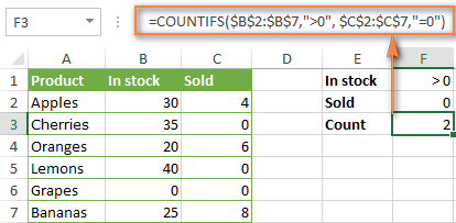
Suppose you have a product list like shown in the screenshot below. You want to get a count of items that are in stock (value in column B is greater than 0) but have not been sold yet (value is column C is equal to 0).
The task can be accomplished by using this formula:
=COUNTIFS(B2:B7,">0", C2:C7,"=0")
And the count is 2 ("Cherries" and "Lemons"):
Formula 2. COUNTIFS formula with two criteria
When you want to count items with identical criteria, you still need to supply each criteria_range / criteria pair individually.
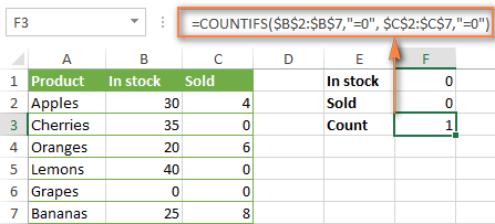
For example, here's the right formula to count items that have 0 both in column B and column C:
=COUNTIFS($B$2:$B$7,"=0", $C$2:$C$7,"=0")
This COUNTIFS formula returns 1 because only "Grapes" have "0" value in both columns.
Using a simpler formula with a single criteria_range like COUNTIFS(B2:C7,"=0") would yield a different result - the total count of cells in the range B2:C7 containing a zero (which is 4 in this example).
How to count cells with multiple criteria (OR logic)
As you have seen in the above examples, counting cells that meet all of the specified criteria is easy because the COUNTIFS function is designed to work this way.
But what if you want to count cells for which at least one of the specified conditions is TRUE, i.e. based on the OR logic? Overall, there are two ways to do this - by adding up several COUNTIF formulas or using a SUM COUNTIFS formula with an array constant.
Formula 1. Add up two or more COUNTIF or COUNITFS formulas
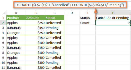
In the table below, supposing you want to count orders with the "Cancelled" and "Pending" status. To have it doen, you can simply write 2 regular Countif formulas and add up the results:
=COUNTIF($C$2:$C$11,"Cancelled") + COUNTIF($C$2:$C$11,"Pending")
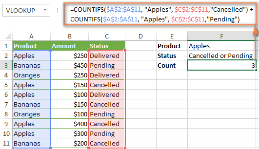
In case each of the functions is supposed to evaluate more than one condition, use COUNTIFS instead of COUNTIF. For example, to get the count of "Cancelled" and "Pending" orders for "Apples" use this formula:
=COUNTIFS($A$2:$A$11, "Apples", $C$2:$C$11,"Cancelled") + COUNTIFS($A$2:$A$11, "Apples", $C$2:$C$11,"Pending")
Formula 2. SUM COUNTIFS with an array constant
In situations when you have to evaluate a lot of criteria, the above approach is not the best way to go because your formula would grow too big in size. To perform the same calculations in a more compact formula, list all of your criteria in an array constant, and supply that array to the criteria argument of the COUNTIFS function. To get the total count, embed COUNTIFS inside the SUM function, like this:
In our sample table, to count orders with the status "Cancelled" or "Pending" or "In transit", the formula would go as follows:
=SUM(COUNTIFS($C$2:$C$11, {"cancelled", "pending", "in transit"}))
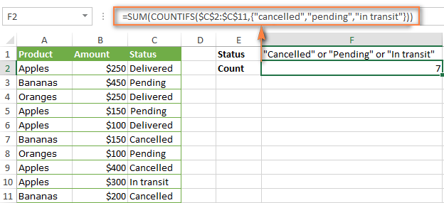
In a similar manner, you can count cells based on two or more criteria_range / criteria pairs. For instance, to get the number of "Apples" orders that are "Cancelled" or "Pending" or "In transit", use this formula:
=SUM(COUNTIFS($A$2:$A$11,"apples",$C$2:$C$11,{"cancelled","pending","in transit"}))

You can find a few more ways to count cells with OR logic in this tutorial: Excel COUNTIF and COUNTIFS with OR conditions.
How to count numbers between 2 specified numbers
By and large, COUNTIFS formulas for numbers fall into 2 categories - based on several conditions (explained in the above examples) and between the two values you specify. The latter can be accomplished in two ways - by using the COUNTIFS function or by subtracting one COUNTIF from another.
Formula 1. COUNTIFS to count cells between two numbers
To find out how many numbers between 5 and 10 (not including 5 and 10) are contained in cells C2 through C10, use this formula:
=COUNTIFS(C2:C10,">5", C2:C10,"<10")
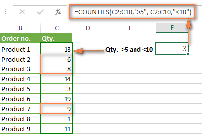
To include 5 and 10 in the count, use the "greater than or equal to" and "less than or equal to" operators:
=COUNTIFS(B2:B10,">=5", B2:B10,"<=10")
Formula 2. COUNTIF formulas to count numbers between X and Y
The same result can be achieved by subtracting one Countif formula from another. The first one counts how many numbers are greater than the lower bound value (5 in this example). The second formula returns the count of numbers that are greater than the upper bound value (10 in this case). The difference between the first and second number is the result you are looking for.
- =COUNTIF(C2:C10,">5")-COUNTIF(C2:C10,">=10") - counts how many numbers greater than 5 and less than 10 are in the range C2:C10. This formula will return the same count as shown in the screenshot above.
- =COUNTIF(C2:C10, ">=5")-COUNTIF(C2:C10, ">10") - the formula counts how many numbers between 5 and 10 are in the range C2:C10, including 5 and 10.
How to use cell references in COUNTIFS formulas
When using logical operators such as ">", "<", "<=" or ">=" together with cell references in your Excel COUNTIFS formulas, remember to enclose the operator in "double quotes" and
add an ampersand (&) before a cell reference to construct a text string.
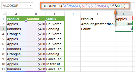
In a sample dataset below, let's count "Apples" orders with amount greater than $200. With criteria_range1 in cells A2:A11 and criteria_range2 in B2:B11, you can use this formula:
=COUNTIFS($A$2:$A$11, "Apples", $B$2:$B$11, ">200")
Or, you can input your criteria values in certain cells, say F1 and F2, and reference those cells in your formula:
=COUNTIFS($A$2:$A$11, $F$1, $B$2:$B$11, ">"&$F$2)
Please notice the use of absolute cell references both in the criteria and criteria_range arguments, which prevents the formula from being broken when copied to other cells.
For more information about the use of an ampersand in COUNTIF and COUNTIFS formulas, please see Excel COUNTIF - frequently asked questions.
How to use COUNTIFS with wildcard characters
In Excel COUNTIFS formulas, you can use the following wildcard characters:
- Question mark (?) - matches any single character, use it to count cells starting and/or ending with certain characters.
- Asterisk (*) - matches any sequence of characters, you use it to count cells containing a specified word or a character(s) as part of the cell's contents.
Tip. If you want to count cells with an actual question mark or asterisk, type a tilde (~) before an asterisk or question mark.
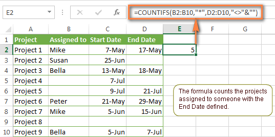
Now let's see how you can use a wildcard char in real-life COUNTIFS formulas in Excel. Suppose, you have a list of projects in column A. You wish to know how many projects are already assigned to someone, i.e. have any name in column B. And because we are learning how to use the COUNTIFS function with multiple criteria, let's add a second condition - the End Date in column D should also be set.
Here is the formula that works a treat:
=COUNTIFS(B2:B10,"*",D2:D10,"<>"&""))
Please note, you cannot use a wildcard character in the 2nd criteria because you have dates rather that text values in column D. That is why, you use the criteria that finds non-blank cells: "<>"&""
COUNTIFS and COUNTIF with multiple criteria for dates
The COUNTIFS and COUNTIF formulas you use for dates are very much similar to the above formulas for numbers.
Example 1. Count dates in a specific date range
To count the dates that fall in a certain date range, you can also use either a COUNTIFS formula with two criteria or a combination of two COUNTIF functions.
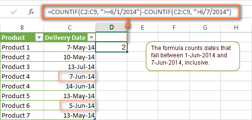
For example, the following formulas count the number of dates in cells C2 through C10 that fall between 1-Jun-2014 and 7-Jun-2014, inclusive:
=COUNTIFS(C2:C9, ">=6/1/2014", C2:C9, "<=6/7/2014")
=COUNTIF(C2:C9, ">=6/1/2014") - COUNTIF(C2:C9, ">6/7/2014")
Example 2. Count dates with multiple conditions
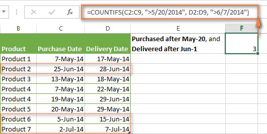
In the same manner, you can use a COUNTIFS formula to count the number of dates in different columns that meet 2 or more conditions. For instance, the below formula will find out how many products were purchased after the 20th of May and delivered after the 1st of June:
=COUNTIFS(C2:C9, ">5/1/2014", D2:D9, ">6/7/2014")
Example 3. Count dates with multiple conditions based on the current date
You can use Excel's TODAY() function in combination with COUNTIF to count dates based on the current date.
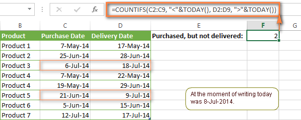
For example, the following COUNTIF formula with two ranges and two criteria will tell you how many products have already been purchased but not delivered yet.
=COUNTIFS(C2:C9, "<"&TODAY(), D2:D9, ">"&TODAY())
This formula allows for many possible variations. For instance, you can tweak it to count how many products were purchased more than a week ago and are not delivered yet:
=COUNTIFS(C2:C9, "<="&TODAY()-7, D2:D9, ">"&TODAY())
This is how you count cells with multiple criteria in Excel. I hope you will find these examples helpful. Anyway, I thank you for reading and hope to see you on our blog next week!
 by
by
1977 comments
How to use Excel COUNTIFS and COUNTIF with multiple criteria on different locations in LAN network
Hi,
i am not able to count using conditions on Different locations, Two files are located on LAN But CountIFS giving ERROR As # Value!
Please Suggest.
Please be more specific. This are no sense.
Expedited Status
Y Approved
N Approved
Y Denied
Y Pended
N Other
N Pended
Y Referred
Y Approved
Y Denied
Count all instances where Expedited is Y and Approved, Denied, or Pended.
I can't figure out a way to do this with out doing a Countifs 3 times. Can you help?
Hello!
Try this:
Make a suplimentary column near column Status.
Use formula in each row (table is starting in A1 cell :) ):
=IF(AND(A2="Y",OR(B2="Approved",B2="Pended",B2="Denied")),1,"")
After that make SUM of column 3 (suplimentary): =SUM(C2:C10)
That is all you need!
It is helpful?
Hi,
Do you know any possibility to format range condidtion in e.g.: countif
following data are given
A1: 001
A2: 002
I'd linke to search for everything less than 2
but countif(value(A1:A2),"<=2") does not work
Any hint would be appreciated highly
Is your data stored as text?
Change to number format.
I have cell data like
(A ) (B)
44201612:33 L
442016 23:33 T
442016 17:33 D
552017 12:33 W
332016 01:33 E
And i have to count only 4-4-2016 date (T)data not with time pls any help thanks in advance
I have cell data like
(A ) (B)
4-4-201612:33 L
4-4-2016 23:33 T
4-4-2016 17:33 D
5-5-2017 12:33 W
3-3-2016 01:33 E
And i have to count only 4-4-2016 date (T)data not with time pls any help thanks in advance
how do I create a formula were age is compared to a range of potential age data which in turn provides a percentage outcome to apply?
age +range =%
=30 =40 =50 59 8.50% 14.500%
Hey!
Can I put multiple criteria for the same range or same criteria on multiple ranges/columns while applying Countifs?
Could you please help me with below problem with multiple criteria:
designation: supervisor, assistant, technician, helper
rating : a, b, c
want to calculate how many (supervisor+ technician) got A & B Rating
and how many got "C" rating.
Regards
Hi,
Could you please tell me how to give multiple conditions
student_no sub1 sub2 sub3
1 p p f
2 p ab f
for this scenario if i want to get details of the no. of subjects failed( which should include absent if any)of each student,
ie for student 2 i should get output as no. of subjects failed = 2, how should i give the condition
i have column A of different gender and in the next column i have their grades and i have to find out that how many boys and man from column A has "a" grade
I would like to set up a formula that looks at a table that includes a column with dates and another column with some binning codes (1a, 1b, 1c, etc). The formual needs to look at the table and count the number of items with the specific text (1a, 1b, 1c, etc) and is between specific dates included in the other column. im not sure which function to use.
I have 2 columns, Unit Type and Status.
In Unit Type its its 1BR and 2BR, In Status its Leased or Blank.
How can i know by function how many 1BR is leased and how many 2BR is Leased.
Unit Type Counts
1BR
2BR
My Dear Svetlana,
Really impressed with your solutions.
I have also one problem. I m having 19.69,19.690,19.691 type series (Text format) in a column of excel and using count if function to calculate the occurrence of 16.69, But it is also including 16.690 in results. whereas i want sepearte figures for 16.690 & 16.69.
Waiting for a solution from you
Hi!
I’m trying to figure out the formula to calculate the following: I want to know how many customers that have made X number of purchases between date Y and Z?
For example: How many customers have made a TWO purchases between 01/04/16 and 01/13/16?
(List of purchases)
A B
1 Date Customer
2 01/02/16 Jack
3 01/04/16 Alice
4 01/05/16 Sam
5 01/07/16 Alice
6 01/09/16 Jack
7 01/13/16 Sam
8 01/17/16 Laura
Many thanks in advance!
/Rickard
Hi!
I am a teacher trying to create a spreadsheet for our grade level. I am trying to count the number of correct answers on a test. Because I want it to be the easiest way for teachers to enter data, I'd like to keep it within the order of the questions (Ex 1-14), however, not all of the questions need to be counted. We are separating them according to "must know" and "extended thinking" type questions. Therefore, there is not always a contiguous range and sometimes it will be a single column. Example Must knows - 1, 4-9, 11, 13, and the extended thinking would be 2,3,10, and 14. There would be separate totals kept for each. Is this at all possible to do with the Countif formula? Thank you!
Is it possible to do a COUNTIF for different date formats? For my work, we indicate contact attempts with the date format of mm/dd/yy and indicate that way made contact with the date format of mm/dd/yyyy. After the initial contact/attempt we use commas and only the mm/dd of the contact/attempt ( We need to track the number of customers we've attempted to contact and the number of customers in which we have actually made contact with. Any formula recommendations?
how can I do this by using formula?
1 1 AHMEDABAD
2 2 AJMER
4 3 BANGALORE
5 4 BARWALA
6 5 BHOPAL
7 6 CHENNAI
8 7 DELHI
11 8 HOSPET
12 9 HYDERABAD
13 10 INDORE
14 11 JABALPUR
15 12 KOLKATA
19 13 MUMBAI
20 14 MYSORE
22 15 NAMAKKAL
24 16 PUNE
25 17 PUNJAB
26 18 RAIPUR
27 19 VIJAYWADA
29 20 WARANGAL
1 AHMEDABAD
2 AJMER
4 BANGALORE
5 BARWALA
6 BHOPAL
7 CHENNAI
8 DELHI
11 HOSPET
12 HYDERABAD
13 INDORE
14 JABALPUR
15 KOLKATA
19 MUMBAI
20 MYSORE
22 NAMAKKAL
24 PUNE
25 PUNJAB
26 RAIPUR
27 VIJAYWADA
29 WARANGAL
Can anyone help me with the above for a formula?
If a cell A contains a number greater than “0” return “red” (this needs to be the primary), if cell B contains a number greater than “0” return Amber (my secondary), or, both cells equal “0” return “Green”
Will Anyone help me to solve this issue.
i want to count specific month and year with two different criteria ("On Work" & "Suspend")
Date Employee Status
28-11-2016 on Work
26-11-2016 suspend
26-11-2016 on work
22-08-2016 on work
27-08-2016 suspend
05-05-2016 Stop work
05-05-2016 Stop work
19-11-2016
Hi
I have this very simple countifs formula and just want to DO an isblank function on the 2nd criteria_range when date isblank in that range.
Sometimes a data in the column range G$2:G$18 is blank and want to replace with Today(). How to I do an isblank on that Range.
eg: if(isblank(G$2:G$18),today(),G$2:G$18)
=COUNTIFS(A$2:A$18,A2,G$2:G$18,"<30/08/2008")
John
Hi, I am not sure which function to use for the following criteria:
Say i have a"closing date" not in order, in column A and corresponding "outcome" in column B. Outcome can be "sold", "refused", "reserved". How to display in the month of November how many "sold", "reserved" and "refused" in different rows. I am not sure how to use the COUNTIF function with a date range and corresponding values in the adjacent column. Please help, Thank you.
It is a misnomer in this article to call the formula a COUNTIF function with OR - as you are adding duplicate values (this should be called AND).
I am working on a dataset and would like to identify patients who had any assisted reproductive technology to become pregnant.
Patients selected yes or no to whether they had surgery, IVF, or prescription medications (in 3 columns). I do not want to count someone who had IVF and prescription meds, for example, as two values. The only way I know how to do this is with a helper column - is there another way?
Thanks!
Hello Jenny,
Excel's COUNTIFS function counts only those cells that meet all of the specified criteria. We call it AND logic, because it is how Excel's AND function works.
If you want to count cells what meet at least one of the specified criteria (any of the specified criteria), add 2 or more COUNTIF functions. We call it OR logic, because Excel's OR function works this way.
As for your task, please be a bit more specific - describe what columns contain what values and what exactly cells you want to count.
Hello I am trying to figure out how to use OR logic with the following formula. I need it to give me a value of 1 if one of the 3 countifs is true.
=COUNTIFS(Table13[CDI],"*110*",Table13[START 1],""&TODAY())
+ COUNTIFS(Table13[CDI],"*110*",Table13[START 2],""&TODAY())
+ COUNTIFS(Table13[CDI],"*110*",Table13[START 3],""&TODAY())
Hi,
I'm currently struggling with making a formula a little more...straight forward and less contrived. I'm currently using this setup:
=COUNTIFS([rangeA], ""&"", [rangeB], =A1, [rangeC], "*entryA*", [rangeC], "*entryB*", [rangeC], "*entryC*", etc.)
The question is this: is there an easier way to exclude multiple entries from the same range?
Thank you.
Hi Svetlana
Would it be possible to use the COUNTIFS function to match two criteria (date and value) and return the date:
For e.g Column G has Bank Codes (up to 3 codes for Bank accounts), Column Q is the date column for which entries appear in the bank account. Column R where formula should be inserted will locate and filter the dates for each bank account so that there's inly one date entry for each bank account
Bank Code(G) Cashbook balance date(Q) Helper(R)
B1 01/04/2016
B1 01/04/2016 01/04/2016
B2 01/04/2016 01/04/2016
B2 03/04/2016 03/04/2016
At the moment, I am using this formula in Column R:
IF(COUNTIF(G$5:G$1048576,[@[Bank Code]]),IF(COUNTIF($Q$5:$Q$1048576,Q5)=COUNTIF($Q$5:Q5,Q5),Q5,""),"")
but it only returns unique dates without considering that there are multiple bank codes.
I would appreciate any help from you.
Thank you.
hi , i want to count Column B text value if Column C have pass value in front of column B's value .
Column B | Column C
------------------------------|
text | pass |
--------------|---------------|
newtext | sent |
------------------------------|
Hello,
I am trying to set up a countifs formula that will count 1 for every time the ocurence of 210 shows up in a column inside a table. my issue is that the cells I am looking through have multiple values that vary per row.
4: 110, 120, 210
5: 13A, 13B, 210
what formula can I use to count how many times 210 has shown up in the tables column?
Try this:
=COUNTIF(A4:A5,"*210*")
Dear Sir/Mam
i am using countifs function with OR logic (formula mentioned below) but it is not working.
=COUNTIFS(HOD,$A26,Non_Moving,BA$7,FSN,"I",Item_Type,OR("NON CRITICAL","OBSLT"))
kindly help me.
hello, I'm struggling with the countifs function.
I'm puttting this in my excel and it gives me an error message all the time!
Do you know what it can be???
=COUNTIFS("E1678:E2515,"=review",M1678:M2515,"<30")
It's killing me!
Hi Hugo,
There is an extra double quote character before E1678:E2515. Once it's removed, your formula works perfectly:
=COUNTIFS(E1678:E2515,"review",M1678:M2515,"<30")
Hello, I am trying to tally the number of rows across multiple worksheets in the same workbook that meet 2 criteria. 1. An X is in a row signifying CRITICAL. 2. Another cell in the same row is blank, meaning the CRITICAL issue was not resolved. =COUNTIFS('AMH:INFO (2)'!E2:E52,"X",'AMH:INFO (2)'!H2:H52,"") is my current formula and it returns #VALUE. I appreciate any help you can give
Lets see this
i have 2 columns with data
like the following
A B
10 10
20 18
16 20
. .
. .
. .
so i want to count how many times the values in column A are greater then the values in column B
is there any countif cobination for that or do i have to add an extra column (C) in wich the diferences betwen A&B are displayed and then use the countif function on column C???
I really want to avoid adding a new column
Can't get this to work =COUNTIF(D4:D154,D165)-COUNTIF(H4:H154,">=K165")-COUNTIF(H4:H154,"<=L165") where column D is my hearing type HESU, HEPS... Column K is my start date (7/1/2016, 8/1/2016..) and Column L is my end date (7/31/2016, 8/31/2016...).
I have two columns. If column A is "Big" and there is a date in column B, it must be counted.
Bus Size Tyre Attendant Week 1
01/10/2016 ~ 09/10/2016
Big
Big
Big 01/10/2016
Big
Big 01/10/2016
Small
Small
Small
Small
Small 01/10/2016
Small
Hi,
I am currently using a formula having hardcoded values:
= SUM(COUNTIFS('Today''s Defects'!G:G,{"New","In Development","In Code Review","In Test","Reopened"},'Today''s Defects'!F:F,"Blocker"))
Now i want to change the values that i am providing to cell references so that whenever i change the value of the cell, automatically it gets reflected in the formula:
= SUM(COUNTIFS('Today''s Defects'!G:G,{D22,C22,E22,R22},'Today''s Defects'!F:F,"Blocker"))
But its not working. Could you please help in this
This site is so helpful! Thanks for everything you post!
I have a basic spreadsheet that lists my employees down column a and across row 1 is every date of the year. I use it to track attendance (they get points if they call in). Is there a way to count the number of blank cells between entries? Their points get cut in half if they go 90 days without an occurrence. Is there a way to make their total points cut in half automatically if there is no occurrence for 90 days?
Thank You
Can someone show me the formula needed to count how many times certain text appears in one column (the text can appear multiple times in one cell or just once) while meeting criteria from another cell.
For Example:
Year Action Taken
2010 Case 1: No Action, Case 2: No Action
2015 Case 1: Suspension, Case 2: Termination
2016 Case 1: No Action
2012 Case 1: Letter, Case 2: Termination
2010 Case 1: Suspension, Case 2: No Action
2010 Case 1: Letter, Case 2: No Action, Case 3: No Action
2013 Case 1: Suspension
I need a formula that will count the number of times in 2010, No Action was taken in cases. The answer is 3.
Please put me out of my misery and tell me how i have 2 sets of COUNTIF's with different criteria
COUNTIF(('Raw Data'!A:A,"1")*('Raw Data'!N:N,"TEXT1")+COUNTIF('Raw Data'!N:N,"TEXT2") ETC
('Raw Data'!A:A,"1") = count of year required
Thanks, Janet
I've tried both a dual added countif (=countif(data!e:e,">=.9")+countif(data!ae:ae,"=true") result 8) and countifs(data!e:e,">=.9",data!ae:ae,"=true") result 0) and neither result was correct (3). I also tried subtracting a countif from a countif (=countif(data!ae:ae,"=true")-countif(data!e:e,"<.9")). I've tried multiple extra parentheses. I'm not sure why this isn't working. One column is a percentage and the other is one of three results: true, false, NA. Can countif(s) not compare different types of data? I thought they could. I can't do a pivot table because some of the devices this file is on can't access data refresh and pivot table creation.
=COUNTIF(D11:F11,"Y")*0.0833+COUNTIF(G11:H11,"Y")*0.1251+COUNTIF(I11:K11,"Y")*0.0833+COUNTIF(L11:O11,"Y")*0.0625
I do a monthly quality assurance on all of my employees and the above formula is what I am using to get a percentage for their monthly score. If you add up all of the percentages it works out to 100% but if a column is not applicable to a specific rep then I need the formula to ignore that cell but still have the rest equal 100%. I have four "Categories" worth a total of 25% each with anywhere from 2-4 subcategories per section. So using the formula above if cell D11 was N/A for the work done for the month I would want cells E11 & F11 to equal 12.5% each instead of 8.33%. Is this possible and if so how? Thank you!
Hi!
I am looking at 700+ text reviews and would like to understand the frequency that any in a set of words are mentioned in a single formula. Is that possible? My current formula is returning too few results (I assume because it is looking for '+'), and I can't seem to make 'OR' work!
Current formula:
=COUNTIF(D3:E716,"food*")+COUNTIF(D3:E716,"cake*")+COUNTIF(D3:E716,"tea*")+COUNTIF(D3:E716,"coffee")+COUNTIF(D3:E716,"restaurant*")+COUNTIF(D3:E716,"*meal*")+COUNTIF(D3:E716,"soup*")+COUNTIF(D3:E716,"lunch*")+COUNTIF(D3:E716,"sandwich")+COUNTIF(D3:E716, "cafe")
In Boolean, I'd simply put:
(food or cake or tea* or coffee or restaurant or meal* or soup* or lunch* or sandwich or cafe) to return ANY mention of these words.
Criteria Range Values
0 5 4
6 10 2
11 15 8
16 20 15
21 25 25
26 30 38
I want to count how many vaules fall in each respective range.
Regards,
Hi Svetlana,
I am trying to count item pairs in the same range (row).
I have tried countifs formulas, but they won't work.
My data looks something like this:
1 A B C D
2 1 12 18 23
3 1 12 20
I would like to count if certain pairs are in a certain row, e.g.:
Does range A2:D2 have 1&12, does it have 1&18, does it have 12&18?
--> in this case excel should return a 3, cause all three pairs are in that row
But for row 3 it should only return 1, cause the pairs 1&18 and 12&18 are not in row 2.
I am greatful for any help I can get.
Thank you for taking the time.
I have a number of words in a row of cells I wish to count but my problem is I cannot get the countifs to count more than one group of cells with in the same formula. Cells contain the words LABPRAC, GAP, GAPVIADISTANCE. Not all cells have a word and no cell has any more than 1 word in it.
example
A1 GAP
A2 GAP
A3 GAPVIADISTANCE
A4 LABPRAC
A5 GAPVIADISTANCE
A6 GAP
A7 LABPRAC
A8 GAPVIADISTANCE
What I am trying to do is add the two words GAP & GAPVIADISTANCE together to give me a total for these to words.
Can you help me as I have tried a few different combinations of the COUNTIFS and SUMIFS formulas but cannot get it to add 2 words from the same cell group together.
Kind regards
I figured it out .....no need to reply thanks
How bro help please
hello Svetlana Cheusheva...which site is useful for learning access 2013
Hello Malaki,
I know very little about MS Access. Anyway, I'd start with this site (support.office.com) as an entry point - it provides a selection of Access 2013 videos and tutorials for Beginner and Intermediate levels.
hello ...u are so helpful God bless you
I want to run a countif on a range of dates based upon today's date -days to pull in last week's data and then the countif would report number of data points from another column.
Column A has dates
Column B has number of days
want to have a formula that days countif "cell =s today" minus 8 days through minus 3 days, then countif number of cells in another columns that are greater than X number.
Thank You
Ted
Hi! I can't seem to get the right answer in using the countif function with two criteria.
I wanted to get the number of a segment with a range of specific score. For example, this is the raw data:
Segment CEET Scores
Starter 40
Adapter 40
Shifter 1 40
Shifter 2 40
Shifter 3 40
Shifter 4 40
Starter 40
Adapter 50
Shifter 1 40
Shifter 2 40
Shifter 3 40
Shifter 4 40
I should get this answer:
Starter with score 40 = 2
Adapter with score 40 = 1
Shifter 1 with score 40 = 2
Shifter 2 with score 40 = 2
Shifter 3 with score 40 = 2
Shifter 4 with score 40 = 2
I'm working with a thousand numbers here.
Hoping you can help me.
Thank you so much! :)
I want to use countif with two ranges of row
condition 1 = font colour red in first
condition 2 = match the content "H" in cell of another row
If the above two condition matches then count.