The tutorial explains how to use COUNTIFS and COUNTIF formulas with multiple criteria in Excel based on AND as well as OR logic. You will find a number of examples for different data types - numbers, dates, text, wildcard characters, non-blank cells and more.
Of all Excel functions, COUNTIFS and COUNTIF are probably most often mixed up because they look very much alike and both are purposed for counting cells based on the specified criteria.
The difference is that COUNTIF is designed for counting cells with a single condition in one range, whereas COUNTIFS can evaluate different criteria in the same or in different ranges. The aim of this tutorial is to demonstrate different approaches and help you choose the most efficient formula for each particular task.
Excel COUNTIFS function - syntax and usage
The Excel COUNTIFS function counts cells across multiple ranges based on one or several conditions. The function is available in Excel 365, 2021, 2019, 2016, 2013, Excel 2010, and Excel 2007, so you can use the below examples in any Excel version.
COUNTIFS syntax
The syntax of the COUNTIFS function is as follows:
- criteria_range1 (required) - defines the first range to which the first condition (criteria1) shall be applied.
- criteria1 (required) - sets the condition in the form of a number, cell reference, text string, expression or another Excel function. The criteria defines which cells shall be counted and can be expressed as 10, "<=32", A6, "sweets".
- [criteria_range2, criteria2]… (optional) - these are additional ranges and their associated criteria. You can specify up to 127 range/criteria pairs in your formulas.
In fact, you don't have to remember the syntax of the COUNTIF function by heart. Microsoft Excel will display the function's arguments as soon as you start typing; the argument you are entering at the moment is highlighted in bold.

Excel COUNTIFS - things to remember!
- You can use the COUNTIFS function in Excel to count cells in a single range with a single condition as well as in multiple ranges with multiple conditions. If the latter, only those cells that meet all of the specified conditions are counted.
- Each additional range must have the same number of rows and columns as the first range (criteria_range1 argument).
- Both contiguous and non-contiguous ranges are allowed.
- If the criteria is a reference to an empty cell, the COUNTIFS function treats it as a zero value (0).
- You can use the wildcard characters in criteria - asterisk (*) and question mark (?). See this example for full details.
How to use COUNTIFS and COUNTIF with multiple criteria in Excel
Below you will find a number of formula examples that demonstrate how to use the COUNTIFS and COUNTIF functions in Excel to evaluate multiple conditions.
How to count cells with multiple criteria (AND logic)
This scenario is the easiest one, since the COUNTIFS function in Excel is designed to count only those cells for which all of the specified conditions are TRUE. We call it the AND logic, because Excel's AND function works this way.
Formula 1. COUNTIFS formula with multiple criteria
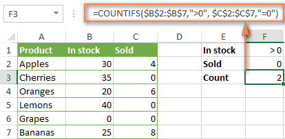
Suppose you have a product list like shown in the screenshot below. You want to get a count of items that are in stock (value in column B is greater than 0) but have not been sold yet (value is column C is equal to 0).
The task can be accomplished by using this formula:
=COUNTIFS(B2:B7,">0", C2:C7,"=0")
And the count is 2 ("Cherries" and "Lemons"):
Formula 2. COUNTIFS formula with two criteria
When you want to count items with identical criteria, you still need to supply each criteria_range / criteria pair individually.
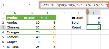
For example, here's the right formula to count items that have 0 both in column B and column C:
=COUNTIFS($B$2:$B$7,"=0", $C$2:$C$7,"=0")
This COUNTIFS formula returns 1 because only "Grapes" have "0" value in both columns.
Using a simpler formula with a single criteria_range like COUNTIFS(B2:C7,"=0") would yield a different result - the total count of cells in the range B2:C7 containing a zero (which is 4 in this example).
How to count cells with multiple criteria (OR logic)
As you have seen in the above examples, counting cells that meet all of the specified criteria is easy because the COUNTIFS function is designed to work this way.
But what if you want to count cells for which at least one of the specified conditions is TRUE, i.e. based on the OR logic? Overall, there are two ways to do this - by adding up several COUNTIF formulas or using a SUM COUNTIFS formula with an array constant.
Formula 1. Add up two or more COUNTIF or COUNITFS formulas
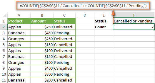
In the table below, supposing you want to count orders with the "Cancelled" and "Pending" status. To have it doen, you can simply write 2 regular Countif formulas and add up the results:
=COUNTIF($C$2:$C$11,"Cancelled") + COUNTIF($C$2:$C$11,"Pending")
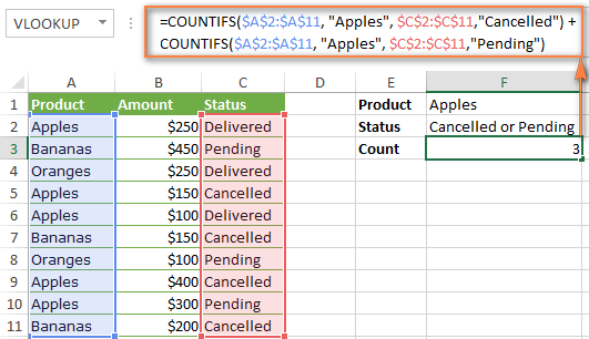
In case each of the functions is supposed to evaluate more than one condition, use COUNTIFS instead of COUNTIF. For example, to get the count of "Cancelled" and "Pending" orders for "Apples" use this formula:
=COUNTIFS($A$2:$A$11, "Apples", $C$2:$C$11,"Cancelled") + COUNTIFS($A$2:$A$11, "Apples", $C$2:$C$11,"Pending")
Formula 2. SUM COUNTIFS with an array constant
In situations when you have to evaluate a lot of criteria, the above approach is not the best way to go because your formula would grow too big in size. To perform the same calculations in a more compact formula, list all of your criteria in an array constant, and supply that array to the criteria argument of the COUNTIFS function. To get the total count, embed COUNTIFS inside the SUM function, like this:
In our sample table, to count orders with the status "Cancelled" or "Pending" or "In transit", the formula would go as follows:
=SUM(COUNTIFS($C$2:$C$11, {"cancelled", "pending", "in transit"}))
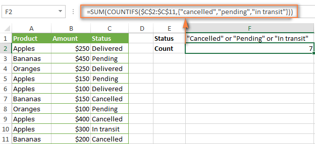
In a similar manner, you can count cells based on two or more criteria_range / criteria pairs. For instance, to get the number of "Apples" orders that are "Cancelled" or "Pending" or "In transit", use this formula:
=SUM(COUNTIFS($A$2:$A$11,"apples",$C$2:$C$11,{"cancelled","pending","in transit"}))

You can find a few more ways to count cells with OR logic in this tutorial: Excel COUNTIF and COUNTIFS with OR conditions.
How to count numbers between 2 specified numbers
By and large, COUNTIFS formulas for numbers fall into 2 categories - based on several conditions (explained in the above examples) and between the two values you specify. The latter can be accomplished in two ways - by using the COUNTIFS function or by subtracting one COUNTIF from another.
Formula 1. COUNTIFS to count cells between two numbers
To find out how many numbers between 5 and 10 (not including 5 and 10) are contained in cells C2 through C10, use this formula:
=COUNTIFS(C2:C10,">5", C2:C10,"<10")
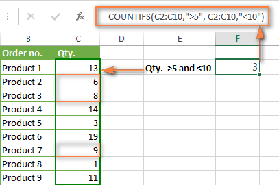
To include 5 and 10 in the count, use the "greater than or equal to" and "less than or equal to" operators:
=COUNTIFS(B2:B10,">=5", B2:B10,"<=10")
Formula 2. COUNTIF formulas to count numbers between X and Y
The same result can be achieved by subtracting one Countif formula from another. The first one counts how many numbers are greater than the lower bound value (5 in this example). The second formula returns the count of numbers that are greater than the upper bound value (10 in this case). The difference between the first and second number is the result you are looking for.
- =COUNTIF(C2:C10,">5")-COUNTIF(C2:C10,">=10") - counts how many numbers greater than 5 and less than 10 are in the range C2:C10. This formula will return the same count as shown in the screenshot above.
- =COUNTIF(C2:C10, ">=5")-COUNTIF(C2:C10, ">10") - the formula counts how many numbers between 5 and 10 are in the range C2:C10, including 5 and 10.
How to use cell references in COUNTIFS formulas
When using logical operators such as ">", "<", "<=" or ">=" together with cell references in your Excel COUNTIFS formulas, remember to enclose the operator in "double quotes" and
add an ampersand (&) before a cell reference to construct a text string.
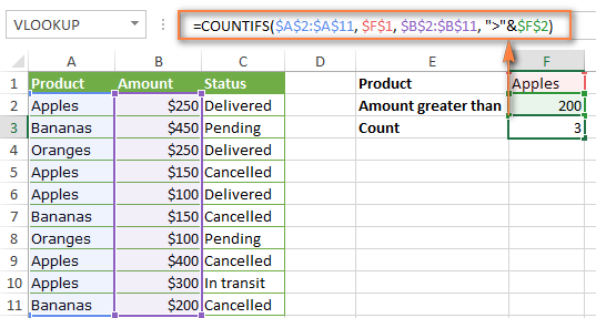
In a sample dataset below, let's count "Apples" orders with amount greater than $200. With criteria_range1 in cells A2:A11 and criteria_range2 in B2:B11, you can use this formula:
=COUNTIFS($A$2:$A$11, "Apples", $B$2:$B$11, ">200")
Or, you can input your criteria values in certain cells, say F1 and F2, and reference those cells in your formula:
=COUNTIFS($A$2:$A$11, $F$1, $B$2:$B$11, ">"&$F$2)
Please notice the use of absolute cell references both in the criteria and criteria_range arguments, which prevents the formula from being broken when copied to other cells.
For more information about the use of an ampersand in COUNTIF and COUNTIFS formulas, please see Excel COUNTIF - frequently asked questions.
How to use COUNTIFS with wildcard characters
In Excel COUNTIFS formulas, you can use the following wildcard characters:
- Question mark (?) - matches any single character, use it to count cells starting and/or ending with certain characters.
- Asterisk (*) - matches any sequence of characters, you use it to count cells containing a specified word or a character(s) as part of the cell's contents.
Tip. If you want to count cells with an actual question mark or asterisk, type a tilde (~) before an asterisk or question mark.
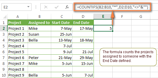
Now let's see how you can use a wildcard char in real-life COUNTIFS formulas in Excel. Suppose, you have a list of projects in column A. You wish to know how many projects are already assigned to someone, i.e. have any name in column B. And because we are learning how to use the COUNTIFS function with multiple criteria, let's add a second condition - the End Date in column D should also be set.
Here is the formula that works a treat:
=COUNTIFS(B2:B10,"*",D2:D10,"<>"&""))
Please note, you cannot use a wildcard character in the 2nd criteria because you have dates rather that text values in column D. That is why, you use the criteria that finds non-blank cells: "<>"&""
COUNTIFS and COUNTIF with multiple criteria for dates
The COUNTIFS and COUNTIF formulas you use for dates are very much similar to the above formulas for numbers.
Example 1. Count dates in a specific date range
To count the dates that fall in a certain date range, you can also use either a COUNTIFS formula with two criteria or a combination of two COUNTIF functions.
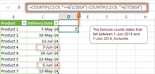
For example, the following formulas count the number of dates in cells C2 through C10 that fall between 1-Jun-2014 and 7-Jun-2014, inclusive:
=COUNTIFS(C2:C9, ">=6/1/2014", C2:C9, "<=6/7/2014")
=COUNTIF(C2:C9, ">=6/1/2014") - COUNTIF(C2:C9, ">6/7/2014")
Example 2. Count dates with multiple conditions
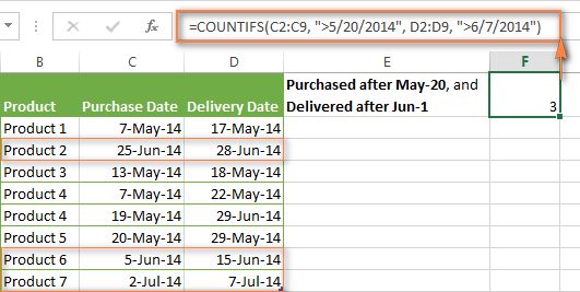
In the same manner, you can use a COUNTIFS formula to count the number of dates in different columns that meet 2 or more conditions. For instance, the below formula will find out how many products were purchased after the 20th of May and delivered after the 1st of June:
=COUNTIFS(C2:C9, ">5/1/2014", D2:D9, ">6/7/2014")
Example 3. Count dates with multiple conditions based on the current date
You can use Excel's TODAY() function in combination with COUNTIF to count dates based on the current date.
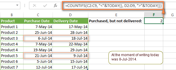
For example, the following COUNTIF formula with two ranges and two criteria will tell you how many products have already been purchased but not delivered yet.
=COUNTIFS(C2:C9, "<"&TODAY(), D2:D9, ">"&TODAY())
This formula allows for many possible variations. For instance, you can tweak it to count how many products were purchased more than a week ago and are not delivered yet:
=COUNTIFS(C2:C9, "<="&TODAY()-7, D2:D9, ">"&TODAY())
This is how you count cells with multiple criteria in Excel. I hope you will find these examples helpful. Anyway, I thank you for reading and hope to see you on our blog next week!
 by
by
1981 comments
Hi
I want to count cells based on two or more criteria_range / criteria pairs. As shown in your example to get the number of "Apples" orders that are "Cancelled" or "Pending" or "In transit".
I copied the data and formula (with correct capitalisation). I get the answer "1" and not "3". The countifs is looking at the first field in the {}. I found this out by altering the order of the data in the {}. This is a problem I was having with my own data and why I am googling the problem. Can you confirm that you still get 3 with the latest version of google sheets.
Apologies this is for excel and not google sheets. Ignore.
how can I count number people with blank columns, e.g. person x in column c has blank cells in column E. I want to count that person has blank cells.
Thanks
I need a formula where it will count the number of dates associated to a company but will only count a date once. For example if a company has 4/8/16,9/8/16,4/8/16,12/16/16, it return 3 for the count and not 4 since 4/8/16 appears twice.
Thank you
I love this site. I always find what I need here. Thank you!
I'm looking for a formula to count all of the information in two separate columns. I've tried everything, but it's not working. My last attempt is: =COUNTIFS(B59:B81, ">=a") + (F59:F81, ">=a")
Hello
I'm trying to figure out a formula that will compare pricing contained in 3 different columns and over 1000 rows, against pricing from 1 column and the same number of rows but then show per cell whether it's value is greater than or less than its respected compared price. Example: in column "B", "C" and "D" there are prices occupying hundreds of rows for those columns. They are to be compared to the prices listed in column "A" for that same row, but to return the values in a "green" or "red" value to signify if it is greater than or less than column "A"s price.
Any ideas?
bb1 = countif($A$1:$B$1,"=2",$A$1:$B$1,"=3") bb2= countif($A$1:$B$1,"=2",$A$1:$B$1,"=4") please tell me how to make this for 20 times . Thank you.
Good afternoon all:
What I would like to do is compare to sets of dates. Column C has the date of when a file was turned in say "1/1/18". Column A has the date of when a file was move into say "12/15/17". I want to see if the difference between the two is more than 16 and how many times that happens. Not sure if this is possible just thought I'd as. Tried the CountIf function but can't figure out the correct criteria.
I have been working on a sales report, that I am needing to get totals by date and name. I have been working on the formula and just can't figure it out. Sample below
5/6/2015 Jason 200.00
5/22/2016 Adam 400.00
1/15/2018 Jason 800.00
4/28/2016 Adam 500.00
4/22/2018 Steve
I have been working on a sales report, that I am needing to get totals by date and name. I have been working on the formula and just can't figure it out. Sample below
Row/Col A B C
1 5/6/2015 Jason 200.00
2 5/22/2016 Adam 400.00
3 1/15/2018 Jason 800.00
4 4/28/2016 Adam 500.00
5 4/22/2018 Steve 200.00
I only want to see the total on sales from 2018 for Jason. How would I write the formula?
This is how I tried, but it is not working
=Countifs(a1:a5,">12/31/2017,b1:b5,"=Jason",Total,"c1:c5")
hello
i am trying to count full day and half day leave for team members
B2 martin
c2 Paid leave d2 1
c3 paid leave d3 0.5
i need a count of martin total leaves taken
eg. Martin 1.5
I am trying to count the number of cells that have a value greater than 100, which have a value of less than 20% in a different column. When I try to use this formula, I get a #Value result. What am I doing wrong?
=COUNTIFS(B1:B726,"20%")
You are so close, forgetting a minor key to major success. ' '
Used int the formula, you'll need it as
=Countif(B2:B726,"<20%")
Stupid Note: I like to use it against decimal values.
Hope you didn't need this in a rush.
HI
how can i Count word and multiple value in excel. for ed
Data Sheet-
Activity Date Topic Like Share View
Facebook 01/01/18 Test 1 1 10
Facebook 01/02/18 Test1 3 1 50
LinkedIn 01/03/18 Test2 4 2 100
Twitter 01/04/18 Test3 9 4 150
Dashboard - Output required like
Post Like - Jan - Feb - Mar - Apr
Facebook
LinkedIn
Twitter
----------------------------------------------------------------------
Need to count facebook like by the facebook posts.
Can you please advise?
- Philip
Hello, Philip,
If I understand your task correctly, please try the following formula:
=SUMIF(A:A,"Facebook",D:D)
Hope it will help you.
Hi there, I am trying to total sales with 2 criteria.
cell:A would have total products sold (1,2,3,4,5)
Cell B will have date order submitted.
I'm trying to add up sum of sales with 3,4, and 5 products sold today().
I've tried a bunch of formulas and I either get #value or 0.
I think I finally figured it out. I ended up using =today() in F12. So now it counts any orders in p29 through p70 that are greater than or equal to 3 and the date listed in u29 through u70 equals todays date.
=COUNTIFS(P29:P70,">=3",U29:U70,F12)
Hi,
Am I able to refer to a cell with text to avoid typing the text? Instead of typing the name in the formula.
Example formula in where F1 and G1 is referencing a cell with my criteria
=COUNTIFS($C$2:$C$21,F1,$D$2:$D$21,G1)
Thank you!!
Hi,
Am I able to refer to a cell with text to avoid typing the text? Instead of typing the name in the formula.
Example formula in where F1 and G1 is referencing a cell with my criteria
=COUNTIFS($C$2:$C$21,F1,$D$2:$D$21,G1)
I am trying to do a formula that involves letters meaning amounts and adding the columns together. How would I do that?
Name - D for diamond or $500, G for Gold or $100, S for Silver or $50.
My columns look like this:
Name 2018 2017 2016 2015 2014 Total
Lesa Sandberg D G S S S $750
I need to know how much money a person has donated over the past years and have it automatically total it. Is this possible? Thanks!
Hello,
Please try the following formula:
=SUMPRODUCT(((B2:G2="D")*500)+((B2:G2="G")*100)+((B2:G2="S")*50))
Hope it will help you.
Seeking a formula:
Currently use:
=countifs((A1:A25),">="&DATE(2017,1,1),(A1:A25),"<="&DATE(2017,1,31))
We now want to select
Q1:Q25 if contains the letter "C" and also fits within the above date ranges...
Please help
Hello,
If I understand your task correctly, please try the following formula:
=COUNTIFS((A1:A25),">="&DATE(2017,1,1),(A1:A25),"<="&DATE(2017,1,31),(Q1:Q25),"=C")
Hope it will help you.
Is there a COUNTIF formula that only counts 1 if the sum of two different cells totals a specific number? I've scoured the web and can't find an answer to this question.
I don't mean the sum of either cells, but only if the two cells added together equal 1. If both cells have 1, I don't want it to count, because the sum of 1 + 1 = 2, and 2 is not 1. For some reason, can't find a formula to count only when ONE of the cells has a 1.
Is there a COUNTIF formula that only counts 1 if the sum of two different cells totals a specific number? I've scoured the web and can't find an answer to this question. I don't mean the sum of either cells, but only if the two cells added together equal 1. If both cells have 1, I don't want it to count, because the sum of 1 + 1 = 2, and 2 is not 1. For some reason, can't find a formula to count only when ONE of the cells has a 1.
How would you type a formula to find out if the sum of two cells is greater than or equal to 3? I tried entering COUNTIFS(A1+M1,"=<3") but was unsuccessful. I need to count multiple pairs of cells, not just one pair at a time.
Thanks
Hello,
Please try the following formula:
=SUMPRODUCT(((A1+M1)<=3)*1)
Hope it will help you.
Data sheet below,
A B
1 Student Name Date
2 Mr. X 11/18/2017
3 Mr. Y 11/18/2017
4 Mr. X 11/20/2017
5 Mr. X 11/25/2017
6 Mr. X 12/21/2017
Above are the details of the persons visiting our office, i want to know, how many times the person Mr. X has visited our office in November only.
Where as the result should be = 3
I am using the below formula...
=COUNTIFS(A2:A6,"Mr. X",B2:B6,">="&DATE(2017,11,1),B2:B6,"<="&DATE(2017,11,31))
But i am getting the result = #VALUE!
Can you please help ......
Hello,
Actually, your formula is correct. If it doesn’t work, then most likely something is wrong with your table.
If you can send me the workbook with your data and formula to support@ablebits.com, I’ll be able to help you better. Please don't worry if you have confidential information there, we never disclose the data we get from our customers and delete it as soon as the problem is resolved.
Don't forget to include the link to this comment into your email.
I'll look into your issue and try to help.
Have you solved your problem?
I have the same issue and i'd like to know the solution for this error "#VALUE!".
Thanks.
I am trying to add the number of Job Titles (Column C) and their Status - Open, Filled (Column B).
I have tried Count if and subtracting the data but it doesn't seem to be working.
=COUNTIF(C11:C67,"CSR",+ B11:B60,"O")
How can I get the number of CSRs that are open between Column C and B?
Hello, Jaime Manale,
Please try the following formula:
=COUNTIFS(C11:C67,"CSR",B11:B67,"O")
Hope it will help you.
I have a formula which is like this
=COUNTIFS('sheet1 '!W:W,">0",'sheet1 '!A:A,"Truck")
which is count all data in column W (sheet1) larger than 0, which are called Truck in column A.
Now, I want this formula to read the same information but by consider a range of dates in between 1st of October to 15th (I have dates in Column B in sheet1).
I now, may I can add to countifs, But not sure about it.
I have one file, it has 3 systems associated to it so it is listed 3 times. Once I have sent all 3 systems for comments I want it to count as 1 as the 1 file has been sent for comments and is complete. So I have currently 1 merged cell for the file and 3 single cells for the systems but I would like it to know when all systems are sent for comments so that I don't need a merged cell, it just counts as 1 once all systems for that filename are sent for comments...not so easy I know but maybe someone can help!
How do I create a formula for the criteria range in a countifs function?
Hello Svetlana
I have 2 columns, 1st contains date and 2nd condition,
I want to count the number of cells contains date range 01-01-2015 to 31-12-2015 with condition A, please help.....
Can the countifs formula count between a date rage with two additional criteria? For example: I have a table that list product by type (industrial, apparel, ect.) in column A, the status (completed, late, on hold, ect.) in column B, and the date entered. I want to be able to count how many apparel products had the late status in June.
Hi
I have a table which shows the gradings for each time estates are inspected ; 'Gold', 'Silver', or 'Bronze'.
I want to know how to count many time the estate rating (Column C) changes from Gold, to Silver or Bronze for each block (column A) on So, for example, on row 9 the estate rating for Ian Mikardo Way, Amersham Road RG4, inspected on 26/06/17, changed from Gold to Silver compared to the previous inspection on 13/04/17.
Thanks for any help you can give
Block (A) Inspection Date(b) Estate Rating (C)
Ian Mikardo Way,
Amersham Road RG4 13/04/2017 Gold
Ian Mikardo Way,
Amersham Road RG4 26/06/2017 Silver
Thanks in advance for whoever can assist
Hi, Kat,
supposing that your table starts from A1, you need to use the following array formula (it should be entered by pressing Ctrl+Shift+Enter on your keyboard instead of just "Enter"):
=SUM($C$2:$C$9*($B$2:$B$9="l")*($A$2:$A$9>=DATEVALUE("9/11/2017"))*($A$2:$A$9<=DATEVALUE("9/26/2017")))
Hope this solves the task!
I'm trying to figure out how to count the following formula:
If an "l" is in the middle column below AND the date falls between 9/11/17 and 9/26/17 sum the amount of the numbers in column 3 that meet the criteria. The information I'm using in below. I've tried several formulas none of which work.
Here are two that I've tried:
1. =COUNTIF(amount,IF(values="l",AND(date,">="&start,"="&start,date,"<="&end+COUNTIF(values,"l"))
The answer should be 29, but if you change the date to a date that is out of range the total does not change, it stays at 29.
date ranges amount
9/10/2017 l 1
9/14/2017 l 2
9/15/2017 m 6
9/10/2012 l 4
9/14/2017 h 3
9/15/2017 l 10
9/9/2017 l 6
9/17/2017 l 8
Good day
i need to count the sum of h7:h21 if d21>0 and then count the sum of h21:h22 if d22>0 and count h22:h52 if d52>0
my problem is that there is no constant cell but constant columns.
The values in the cells in column d will always vary.
can you please assist.
On sheet one I have date joined organisation followed by benefit claimed.
One sheet 2 I have the quarterly date range that I need totals for.
Say Date joined is column A sheet 1, Benefit is column B sheet 1
Date I'm calculating from is cell A1 sheet 2 and Date to is cell A2, sheet 2
I need to know how I can calculate the number of times a specific benefit (say EI or JSA) is listed for people who have joined the organisation within the set date parameters on sheet 2.
Please help!
Hi ,
I am trying to find a count of a particular Number or Letter in a row , i am writing the query but its giving me 0...can you advise
Hi ,
I am trying to find a count of a particular Numnber or Letter in a row , i am writing the query but its giving me 0...can you advsie
I am a desperate beginner and am very "stuck"
BACKGROUND
STEP 1: I have counted 300 trees in our settlement. Each tree was listed by species in Column B. Each tree's health was rated on a scale of 1-5 ion column E.
STEP 2:
I was able to countif and identified 25 species.
MY QUESTION
I want to learn, by species, how many received each health rating, the scale of 1-5.
I think I need countifs, but cannot make that work. Please please help me. Thanks
I have read a book and viewed tutorials, so have tried hard to figure this out on my own.
Hi
I wanted to count in Column "C" when two conditions are met from column "A" and Column "B", like A:A="W" and B:B="KK" count from row "C". Data is
Freq Name Value
D KK 3
D KK 3
D LL 3
W KK 3
W LL 3
Hi, Junaid,
you can try this one:
=COUNTIFS(A2:A6,"W",B2:B6,"KK")
if you take a closer look at this point of the article above, you'll understand how the part of the formula works.
Thanks I got much help nothing words to express
Hi!
I am trying to count two things. (1) which of my customers from January ordered more boxes in February than in January, but excluding customers from February who were not customers in January. Cells a2:a51 list all my customers by name. Cells b2:b51 lists the amount of boxes purchased in January. Cells c2:c51 lists the amount of boxes purchased in February. When using Countifs, I can't figure out how to make the Criteria conditional. I tried using: =countifs(b:2:b51,">0",b:2:b51,">a2:a51"), but that doesn't seem to work. Any advice?
(2) Count the number of customers I lost in February (i.e. customers who purchased boxes in January but none in February). I tried =countifs(a2:a51,">0",b2:b51,"<1") I noticed that works if I have a 0 value in the b2:b51 range. Any way I can make the count work if the value in column b is Blank?
Thank you!!
hi mam if we have age and gender in a single cell how can we count only gender out of it please help me out.i mean only male or female
Trying to add countifs from two sheets in a workbook to a third sheet in the same workbook but I get zero.
Function below.
=COUNTIFS('sheet1 Data'!$A:$A,Tracker!A3,'sheet1 Data'!$J:$J,Tracker!C$2)+COUNTIFS('sheet2 Data'!$A:$A,Tracker!A3,'sheet2 Data'!$J:$J,Tracker!C$2)
Column A represent Date Range
Cell A3 represents the date value
Column C represent Value Range
Cell C2 represents the value
Hi!
Never mind. Function is working.. thank you.
Hi, Can I refer to a cell with text to avoid typing the text for a second condition? Instead of typing the name of employees that match, I'd like to refer to a cell with that name, so I can copy and paste the formula for the names of the other employees. I hope you understand what I need! thanks
Tomás
Sorry, my mistake! it can be done without any problem!! sorry again.
I am to insert serial number to each output (tick mark only) which is a result of this formula; =IF(AND(E11>=1,F11=0),"a",""). The formula is a output for those households whose educational credentials meets my requirements. And I pick those households for my selection. Those with "Nil" output need not count as they are not necessary.
Regards
Can i use criteria average with criteria sum in rule if
I have some workers' salaries and I want to use a class to find out how many classes are in the category of 200, how many are in the category of 100, how many are in the category of 50, how many are in the category of 20, how many are in the category of 10, 5 and how many of the 1 category
Hi !
I need help with the following report :
Status ColoumnA ColoumnB ColoumnC
Prd.sold A c
On hold B
Prd.Tran A
Prd.sold B
I need to understand whether can we use countif condition to check how many prod.sold and On hold customers have opted for ColoumnA product ?
=SUM(COUNTIFS(A2:A8,{"Prd.Sold","OnHold"},B2:B8,"A"))
Hi!
Following is one of the report formats that i need help with :
Status ColoumnA ColoumnB
Hi
I have a spread sheet that consist of a reporting period, a document type and a keyword.
I am trying to do a bar graph that auto changes when information is added.
reporting period is 2017-Q1, 2017-Q2, the document type will always be "Initial Event Notification" and the Keywords are what need to be counted : near miss, injury, breach.
so i figured out the below is the info i am wanting.
countif reporting period = (2017-Q1) & document type = (Initial Event Notification) & keyword = (Injury).
I just havent used excel formulas for a while and am not getting my head around it today.
Hello, can you please help me with this. Im trying to find a formula when "open" is entered in example cell B1 it would calculate the date + 2 days entered in a1 in c3.
Hi Kay,
Here you go:
=IF(B1="open", A1+2)
If the date does not display correctly in the formula cell, be sure to set the desired Date format to it.
Okay I have a survey where respondents can check multiple boxes of various errors found. When it imported into excel it puts these responses into one cell for each case under one column.
One case entry can have multiple categorical answers (or no findings at all) all located on a single cell. Example: Not addressing OWL or NHL screens; Failed to explain how income was calculated; Actual versus Anticipated
I am needing to be able to just look at each piece individually, for example just the Actual versus Anticipated. How do I do a count were it will identify that answer. Right now all I am identifying is when it was the only finding selected. It is not picking up and counting that answer when multiple items have been selected.
Please help!!!!
Hello,
I need a formula linke
=COUNTIF($C$2:$C$11,"Apple") + COUNTIF($C$2:$C$11,"5Orange")
but I need to count the "5Orange" as 5 not 1.
For example if I have in A2 Apple and in B2 5Orange, I want the formula to give me the result of 6.
Is there anyway I could could count the 5Orange as 5.
=COUNTIF($C$2:$C$11,"Apple") + (5*COUNTIF($C$2:$C$11,"5Orange"))
Good Morning,
I need a countifs function that allows me to compare two columns of data and count how many time one words is associated with a word in the first column. Basically I need to count how many people in a particular company have the title "director" but my list is of 1,000 companies. So, if column A is company and Column B are the varying titles, I need to know for each company how many directors they have based off the titles listed in B.
I feel like I will need some kind of array formula? Maybe Vlookup too? idk
PLEASE HELP :)
Sorry seems like posted several times. Apologise.
Dear Svetlana,
Greetings, we meet again. I was trying to put a formula by using COUNTIFS, but it is coming with Error that too many arguments. Can you please advise.
A B C
Details Payment Authority to Waive
Bill 5000 If the value in B2 is less than 5000 then it will
show Manager, more than 5000 it will show General
Manager, more than 10000 it will show Director.
Late Fine 6000 The values will select/show and will show Manager
Total 11000 The values will select/show and will show Director
Thank you for the advise. Have a nice day.
Kaiser
This can be solved by IF function (not CountIF).