Microsoft Excel provides several functions purposed for counting different kinds of cells, such as blanks or non-blanks, with number, date or text values, containing specific words or character, etc.
In this article, we will focus on the Excel COUNTIF function that is purposed for counting cells with the condition you specify. First, we will briefly cover the syntax and general usage, and then I provide a number of examples and warn about possible quirks when using this function with multiple criteria and specific types of cells.
In essence, COUNTIF formulas are identical in all Excel versions, so you can use the examples from this tutorial in Excel 365, 2021, 2019, 2016, 2013, 2010 and 2007.
COUNTIF function in Excel - syntax and usage
Excel COUNTIF function is used for counting cells within a specified range that meet a certain criterion, or condition.
For example, you can write a COUNTIF formula to find out how many cells in your worksheet contain a number greater than or less than the number you specify. Another typical use of COUNTIF in Excel is for counting cells with a specific word or starting with a particular letter(s).
The syntax of the COUNTIF function is very simple:
As you see, there are only 2 arguments, both of which are required:
- range - defines one or several cells to count. You put the range in a formula like you usually do in Excel, e.g. A1:A20.
- criteria - defines the condition that tells the function which cells to count. It can be a number, text string, cell reference or expression. For instance, you can use the criteria like these: "10", A2, ">=10", "some text".
And here is the simplest example of Excel COUNTIF function. What you see in the image below is the list of the best tennis players for the last 14 years. The formula =COUNTIF(C2:C15,"Roger Federer") counts how many times Roger Federer's name is on the list:
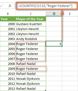
Note. A criterion is case insensitive, meaning that if you type "roger federer" as the criteria in the above formula, this will produce the same result.
Excel COUNTIF function examples
As you have just seen, the syntax of the COUNTIF function is very simple. However, it allows for many possible variations of the criteria, including wildcard characters, the values of other cells, and even other Excel functions. This diversity makes the COUNTIF function really powerful and fit for many tasks, as you will see in the examples that follow.
COUNTIF formula for text and numbers (exact match)
In fact, we discussed the COUNTIF function that counts text values matching a specified criterion exactly a moment ago. Let me remind you that formula for cells containing an exact string of text: =COUNTIF(C2:C15,"Roger Federer"). So, you enter:
- A range as the first parameter;
- A comma as the delimiter;
- A word or several words enclosed in quotes as the criteria.
Instead of typing text, you can use a reference to any cell containing that word or words and get absolutely the same results, e.g. =COUNTIF(C1:C9,C7).
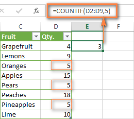
Similarly, COUNTIF formulas work for numbers. As shown in the screenshot below, the below formula perfectly counts cells with quantity 5 in Column D:
=COUNTIF(D2:D9, 5)
In this article, you will find a few more formulas to count cells that contain any text, specific characters or only filtered cells.
COUNTIF formulas with wildcard characters (partial match)
In case your Excel data include several variations of the keyword(s) you want to count, then you can use a wildcard character to count all the cells containing a certain word, phrase or letters as part of the cell's contents.
Suppose, you have a list of tasks assigned to different persons, and you want to know the number of tasks assigned to Danny Brown. Because Danny's name is written in several different ways, we enter "*Brown*" as the search criteria =COUNTIF(D2:D10, "*Brown*").
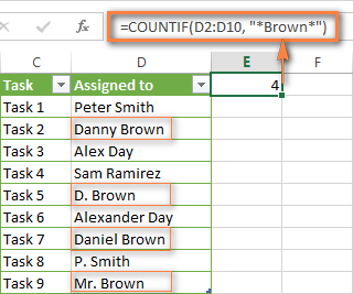
An asterisk (*) is used to find cells with any sequence of leading and trailing characters, as illustrated in the above example. If you need to match any single character, enter a question mark (?) instead, as demonstrated below.
Tip. It is also possible to use wildcards with cell references with the help of the concatenation operator (&). For example, instead of supplying "*Brown*" directly in the formula, you can type it in some cell, say F1, and use the following formula to count cells containing "Brown": =COUNTIF(D2:D10, "*"&F1&"*")
Count cells beginning or ending with certain characters
You can use either wildcard character, asterisk (*) or question mark (?), with the criterion depending on which exactly result you want to achieve.
If you want to know the number of cells that start or end with certain text no matter how many other characters a cell contains, use these formulas:
=COUNTIF(C2:C10,"Mr*") - count cells that begin with "Mr".
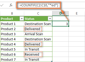
=COUNTIF(C2:C10,"*ed") - count cells that end with the letters "ed".
The image below demonstrates the second formula in action:
If you are looking for a count of cells that start or end with certain letters and contain the exact number of characters, you use the Excel COUNTIF function with the question mark character (?) in the criteria:
=COUNTIF(D2:D9,"??own") - counts the number of cells ending with the letters "own" and having exactly 5 characters in cells D2 through D9, including spaces.
=COUNTIF(D2:D9,"Mr??????") - counts the number of cells starting with the letters "Mr" and having exactly 8 characters in cells D2 through D9, including spaces.
Tip. To find the number of cells containing an actual question mark or asterisk, type a tilde (~) before the ? or * character in the formula. For example, =COUNTIF(D2:D9,"*~?*") will count all cells containing the question mark in the range D2:D9.
Excel COUNTIF for blank and non-blank cells
These formula examples demonstrate how you can use the COUNTIF function in Excel to count the number of empty or non-empty cells in a specified range.
COUNTIF not blank
In some Excel COUNTIF tutorials and other online resources, you may come across formulas for counting non-blank cells in Excel similar to this one:
=COUNTIF(A1:A10,"*")
But the fact is, the above formula counts only cells containing any text values including empty strings, meaning that cells with dates and numbers will be treated as blank cells and not included in the count!
If you need a universal COUNTIF formula for counting all non-blank cells in a specified range, here you go:
Or
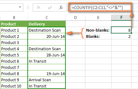
This formula works correctly with all value types - text, dates and numbers - as you can see in the screenshot below.
COUNTIF blank
If you want the opposite, i.e. count blank cells in a certain range, you should adhere to the same approach - use a formula with a wildcard character for text values and with the "" criteria to count all empty cells.
Formula to count cells not containing any text:
Since an asterisk (*) matches any sequence of text characters, the formula counts cells not equal to *, i.e. not containing any text in the specified range.
Universal COUNTIF formula for blanks (all value types):
The above formula correctly handles numbers, dates and text values. For example, here's how you can get the number of empty cells in the range C2:C11:
=COUNTIF(C2:C11,"")
Please be aware that Microsoft Excel has another function for counting blank cells, COUNTBLANK. For instance, the following formulas will produce exactly the same results as the COUNTIF formulas you see in the screenshot above:
Count blanks:
=COUNTBLANK(C2:C11)
Count non-blanks:
=ROWS(C2:C11)*COLUMNS(C2:C11)-COUNTBLANK(C2:C11)
Also, please keep in mind that both COUNTIF and COUNTBLANK count cells with empty strings that only look blank. If you do not want to treat such cells as blanks, use "=" for criteria. For example:
=COUNTIF(C2:C11,"=")
For more information about counting blanks and not blanks in Excel, please see:
COUNTIF greater than, less than or equal to
To count cells with values greater than, less than or equal to the number you specify, you simply add a corresponding operator to the criteria, as shown in the table below.
Please pay attention that in COUNTIF formulas, an operator with a number are always enclosed in quotes.
| Criteria | Formula Example | Description |
|---|---|---|
| Count if greater than | =COUNTIF(A2:A10,">5") | Count cells where value is greater than 5. |
| Count if less than | =COUNTIF(A2:A10,"<5") | Count cells with values less than 5. |
| Count if equal to | =COUNTIF(A2:A10,"=5") | Count cells where value is equal to 5. |
| Count if not equal to | =COUNTIF(A2:A10,"<>5") | Count cells where value is not equal to 5. |
| Count if greater than or equal to | =COUNTIF(C2:C8,">=5") | Count cells where value is greater than or equal to 5. |
| Count if less than or equal to | =COUNTIF(C2:C8,"<=5") | Count cells where value is less than or equal to 5. |
You can also use all of the above formulas to count cells based on another cell value, you will just need to replace the number in the criteria with a cell reference.
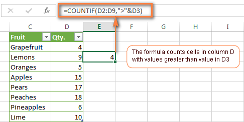
Note. In case of a cell reference, you have to enclose the operator in quotes and add an ampersand (&) before the cell reference. For example, to count cells in the range D2:D9 with values greater than a value in cell D3, you use this formula =COUNTIF(D2:D9,">"&D3):
If you want to count cells that contain an actual operator as part of the cell's contents, i.e. the characters ">", "<" or "=", then use a wildcard character with the operator in the criteria. Such criteria will be treated as a text string rather than a numeric expression. For example, the formula =COUNTIF(D2:D9,"*>5*") will count all cells in the range D2:D9 with contents like this "Delivery >5 days" or ">5 available".
Using Excel COUNTIF function with dates
If you want to count cells with dates that are greater than, less than or equal to the date you specify or date in another cell, you proceed in the already familiar way using formulas similar to the ones we discussed a moment ago. All of the above formulas work for dates as well as for numbers. Let me give you just a few examples:
| Criteria | Formula Example | Description |
|---|---|---|
| Count dates equal to the specified date. | =COUNTIF(B2:B10,"6/1/2014") | Counts the number of cells in the range B2:B10 with the date 1-Jun-2014. |
| Count dates greater than or equal to another date. | =COUNTIF(B2:B10,">=6/1/2014") | Count the number of cells in the range B2:B10 with a date greater than or equal to 6/1/2014. |
| Count dates greater than or equal to a date in another cell, minus x days. | =COUNTIF(B2:B10,">="&B2-"7") | Count the number of cells in the range B2:B10 with a date greater than or equal to the date in B2 minus 7 days. |
Apart from these common usages, you can utilize the COUNTIF function in conjunction with specific Excel Date and Time functions such as TODAY() to count cells based on the current date.
| Criteria | Formula Example |
|---|---|
| Count dates equal to the current date. | =COUNTIF(A2:A10,TODAY()) |
| Count dates prior to the current date, i.e. less than today. | =COUNTIF(A2:A10,"<"&TODAY()) |
| Count dates after the current date, i.e. greater than today. | =COUNTIF(A2:A10,">"&TODAY()) |
| Count dates that are due in a week. | =COUNTIF(A2:A10,"="&TODAY()+7) |
| Count dates in a specific date range. | =COUNTIF(B2:B10, ">=6/1/2014")-COUNTIF(B2:B10, ">6/7/2014") |
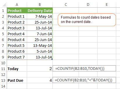
Here is an example of using such formulas on real data (at the moment of writing today was 25-Jun-2014):
Excel COUNTIF with multiple criteria
In fact, Excel COUNTIF function is not exactly designed to count cells with multiple criteria. In most cases, you'd use its plural counterpart, the COUNTIFS function to count cells that match two or more criteria (AND logic). However, some tasks can be solved by combining two or more COUNTIF functions in one formula.
Count values between two numbers
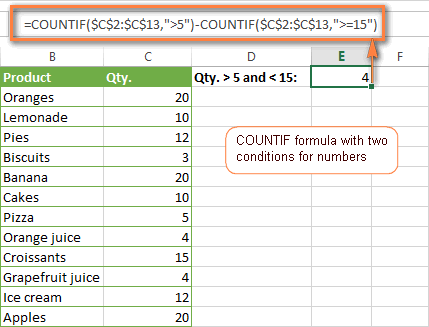
One of the most common applications of Excel COUNTIF function with 2 criteria is counting numbers within a specific range, i.e. less than X but greater than Y. For example, you can use the following formula to count cells in the range B2:B9 where a value is greater than 5 and less than 15.
=COUNTIF(B2:B9,">5")-COUNTIF(B2:B9,">=15")
How this formula works:
Here, we use two separate COUNTIF functions - the first one finds out how many values are greater than 5 and the other one gets a count of values greater than or equal to 15. Then, you subtract the latter from the former and get the desired result.
Count cells with multiple OR criteria
In situations when you want to get several different items in a range, add 2 or more COUNTIF functions together. Supposing, you have a shopping list and you want to find out how many soft drinks are included. To have it done, use a formula similar to this:
=COUNTIF(B2:B13,"Lemonade")+COUNTIF(B2:B13,"*juice")
Please pay attention that we've included the wildcard character (*) in the second criterion, it is used to count all kinds of juice on the list.
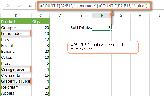
In the same manner, you can write a COUNTIF formula with several conditions. Here is an example of the COUNTIF formula with multiple OR conditions that counts lemonade, juice and ice cream:
=COUNTIF(B2:B13,"Lemonade") + COUNTIF(B2:B13,"*juice") + COUNTIF(B2:B13,"Ice cream")
For other ways to count cells with OR logic, please see this tutorial: Excel COUNTIF and COUNTIFS with OR conditions.
Using COUNTIF function to find duplicates and unique values
Another possible usage of the COUNTIF function in Excel is for finding duplicates in one column, between two columns, or in a row.
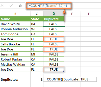
Example 1. Find and count duplicates in 1 column
For example, this simple formula =COUNTIF(B2:B10,B2)>1 will spot all duplicate entries in the range B2:B10 while another function =COUNTIF(B2:B10,TRUE) will tell you how many dupes are there:
Example 2. Count duplicates between two columns
If you have two separate lists, say lists of names in columns B and C, and you want to know how many names appear in both columns, you can use Excel COUNTIF in combination with the SUMPRODUCT function to count duplicates:
=SUMPRODUCT((COUNTIF(B2:B1000,C2:C1000)>0)*(C2:C1000<>""))
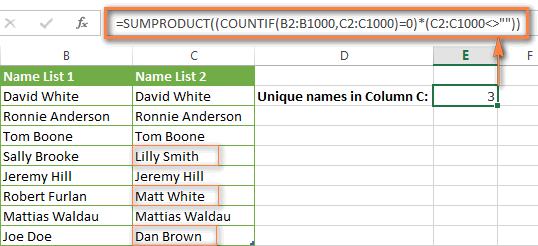
We can even take a step further and count how many unique names there are in Column C, i.e. names that do NOT appear in Column B:
=SUMPRODUCT((COUNTIF(B2:B1000,C2:C1000)=0)*(C2:C1000<>""))
Tip. If you want to highlight duplicate cells or entire rows containing duplicate entries, you can create conditional formatting rules based on the COUNTIF formulas, as demonstrated in this tutorial - Excel conditional formatting formulas to highlight duplicates.
Example 3. Count duplicates and unique values in a row
If you want to count duplicates or unique values in a certain row rather than a column, use one of the below formulas. These formulas might be helpful, say, to analyze the lottery draw history.
Count duplicates in a row:
=SUMPRODUCT((COUNTIF(A2:I2,A2:I2)>1)*(A2:I2<>""))
Count unique values in a row:
=SUMPRODUCT((COUNTIF(A2:I2,A2:I2)=1)*(A2:I2<>""))

Excel COUNTIF - frequently asked questions and issues
I hope these examples have helped you to get a feel for the Excel COUNTIF function. If you've tried any of the above formulas on your data and were not able to get them to work or are having a problem with the formula you created, please look through the following 5 most common issues. There is a good chance that you will find the answer or a helpful tip there.
1. COUNTIF on a non-contiguous range of cells
Question: How can I use COUNTIF in Excel on a non-contiguous range or a selection of cells?
Answer: Excel COUNTIF does not work on non-adjacent ranges, nor does its syntax allow specifying several individual cells as the first parameter. Instead, you can use a combination of several COUNTIF functions:
Wrong: =COUNTIF(A2,B3,C4,">0")
Right: =COUNTIF(A2,">0") + COUNTIF(B3,">0") + COUNTIF(C4,">0")
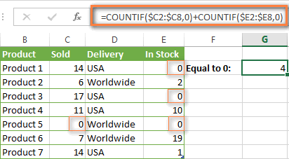
An alternative way is using the INDIRECT function to create an array of ranges. For example, both of the below formulas produce the same result you see in the screenshot:
=SUM(COUNTIF(INDIRECT({"B2:B8","D2:C8"}),"=0"))
=COUNTIF($B2:$B8,0) + COUNTIF($C2:$C8,0)
2. Ampersand and quotes in COUNTIF formulas
Question: When do I need to use an ampersand in a COUNTIF formula?
Answer: It is probably the trickiest part of the COUNTIF function, which I personally find very confusing. Though if you give it some thought, you'll see the reasoning behind it - an ampersand and quotes are needed to construct a text string for the argument. So, you can adhere to these rules:
If you use a number or a cell reference in the exact match criteria, you need neither ampersand nor quotes. For example:
=COUNTIF(A1:A10,10)
or
=COUNTIF(A1:A10,C1)
If your criteria includes text, wildcard character or logical operator with a number, enclose it in quotes. For example:
=COUNTIF(A2:A10,"lemons")
or
=COUNTIF(A2:A10,"*") or =COUNTIF(A2:A10,">5")
In case your criteria is an expression with a cell reference or another Excel function, you have to use the quotes ("") to start a text string and ampersand (&) to concatenate and finish the string off. For example:
=COUNTIF(A2:A10,">"&D2)
or
=COUNTIF(A2:A10,"<="&TODAY())
If you are in doubt whether an ampersand is needed or not, try out both ways. In most cases an ampersand works just fine, e.g. both of the below formulas work equally well.
=COUNTIF(C2:C8,"<=5")
and
=COUNTIF(C2:C8,"<="&5)
3. COUNTIF for formatted (color coded) cells
Question: How do I count cells by fill or font color rather than by values?
Answer: Regrettably, the syntax of the Excel COUNTIF function does not allow using formats as the condition. The only possible way to count or sum cells based on their color is using a macro, or more precisely an Excel User-Defined function. You can find the code working for cells colored manually as well as for conditionally formatted cells in this article - How to count and sum Excel cells by fill and font color.
4. #NAME? error in the COUNTIF formula
Issue: My COUNTIF formula throws a #NAME? error. How can I get it fixed?
Answer: Most likely, you have supplied an incorrect range to the formula. Please check out point 1 above.
5. Excel COUNTIF formula not working
Issue: My COUNTIF formula is not working! What have I done wrong?
Answer: If you have written a formula which is seemingly correct but it does not work or produces a wrong result, start by checking the most obvious things such as a range, conditions, cell references, use of ampersand and quotes.
Be very careful with using spaces in a COUNTIF formula. When creating one of the formulas for this article I was on the verge of pulling my hair out because the correct formula (I knew with certainty it was right!) wouldn't work. As it turned out, the problem was in a measly space somewhere in between, argh... For instance, look at this formula:
=COUNTIF(B2:B13," Lemonade").
At first sight, there is nothing wrong about it, except for an extra space after the opening quotation mark. Microsoft Excel will swallow the formula just fine without an error message, warning or any other indication, assuming you really want to count cells containing the word 'Lemonade' and a leading space.
If you use the COUNTIF function with multiple criteria, split the formula into several pieces and verify each function individually.
And this is all for today. In the next article, we will explore several ways to count cells in Excel with multiple conditions. Hope to see you next week and thanks for reading!
 by
by
1034 comments
i have data of 500 employee ID's with different tasks. I want to use the function countif to get the no of tasks per employee id in mass, it is possible please help me
Please help me i want to calculate electricity rate in excel
Example:
Sr. No House no Name Meter reading
1 1 ABC 50
2 2 XYZ 56
Criteria is if reading 0 to 50 then 0 rs charges if reading >50 but 100 but 150 then 4 rs charges.
Qty. Rate
2 699
1 899
1 809
2 539
1 719
1 539
3 685
1 539
More then 599 and lees or equal to 799
I require output : 6
Detail .
(699 -> 2)+(719 -> 1) +(685 -> 3) = 6
Qty. Rate
2 699
1 899
1 809
2 539
1 719
1 539
3 685
1 539
I use
=COUNTIFS(A:A,">599",A:A," 2)+(719 -> 1) +(685 -> 3) = 6
hi i was wondering if you can use the countif function with a cell reference as part of the criteria. basically instead of saying =countif(Range,"<5") rather saying =countif(range,"<A7"). your help would be greatly appreciated.
thanks
Gavin
A B C D E F G H I J
B 1 0 1 1 1 0 1 1 1
C 0 1 0 0 0 1 0 0 0
D 0 0 1 1 0 0 1 0 1
E 1 1 1 0 1 1 0 1 0
F 0 1 0 1 0 0 1 0 1
G 0 0 1 0 0 1 0 0 0
H 1 0 0 1 1 0 1 1 1
I 0 1 1 0 0 0 0 0 1
J 1 0 1 1 1 1 1 1 0
find duplicate column..
highlight it
Help me with this...
can anyone help me with this ??
i can find the duplicates column in alphabetic mode but i can't in numeric mode
please help me out with this
What about count if greater than 5 and less than 8 for example? or between something?
Hi Khamkeo,
In this case, you need to use the COUNTIFS function, for example:
=COUNTIFS(A2:A10,">5", A2:A10,"<8")
i need help: I have a leads excel (clients) and i plan to calculate how many leads we got:
-yesterday
-today
-last7days
-this month
I have P column that have "7" standard possible answers; like the state of the lead. I need a formula for each state of the lead to count the nr of leads for the above time periods.
Thanks,
I really appreciate this answer i tried for one week to do it.
Hi,
I need help, if I have same words from sheet 1, and i want to count the words in 6 rows in sheet 2. how?
e.g.
sheet 1 - ABC (AE1) criteria
Sheet 2 - A1-F1 range
By using countif formula.
once i put the this formula:COUNIF('Sheet1'!AE1,"*ABC*")
but it is calculating multiple.
Hi, I am having a problem counting how many part numbers with shortages on a multiple data. See below data:
YV756A YV756B YV441G YT081A YT081B
4100023-003 -1 0 -1 -1 -1
4100024-001 0 0 0 0 -1
4100142-001 -1 -1 -1 -1 -1
Need to count how many part number with shortage on following models:
YV756 =
YV441 =
YT081 =
this is considering if YV756A and YV756B has -1 on each, it will take only as 1 part number with shortage.
Please help me create formula to count this.
thanks a lot!
Jenna
I WANT TO COUNT WITH IF BUT AT NEGATIVE
EXMPL
SUMIF -> IF ISNT "THIS"
?
Hi Greg,
You can use the "not equal to" operator (<>) e.g.:
=COUNTIF(A1:A10, "<>"&5)
=COUNTIF(A1:A10, "<>"&"text")
Sir
COUNTIF(G7:G315,"SC") is 38
and I want to count How many R is entered in the next column exact SC means in column H7:H315. pl do the needful and Give formula
I need help counting unique invoices touched by the collector per work day. I used If(I1=I2,0,1) but still getting some duplicate invoices for others. I need column I to give the count of unique invoices touched that day.
Thanks,
JM
Hello!
Please check out the following tutorial, hopefully you will find a proper formula for your task there:
How to count distinct and unique values in Excel
I need a formula to get the total count of non empty columns in excel which is having "n" number of columns.
Ok I have bee through a few help forums now and got tired of searching. I was trying to utilize a Countifs formula to determine employees available to work during certain time frames. Due to the way our system exports the information, an excel formula would work best. Here is how info is exported to excel:
A B C D E F
Name From To Sun Mon Tue
Employee 13:00 00:00 TRUE TRUE FALSE
What I need to do is count how many employees are available during certain times each day, example:
Time Sun Mon Tue
1pm-7pm 1 1 0
Any assistance would be greatly appreciated cause this type of formula is not my strong suit.
Thank you for the simple clear detailed information.
You are an angel.
Hi, how do I count the number of cells in a range that are bigger than 0?
The numbers in the cells are the results of formulas though.
Thanks for your help.
Hi there,
I have a complex spreadsheet and I want to have a formula calculating the following:
From a range of cells to take a particular value (name) and then from another range of cells (column) to take another value matching the row with the name, then to count the matches in the cell.
I have tried this formula
=IF(AND('Domain 1'!E6="Andrea",'Domain 1'!Q6="Food"),1,0)
but the thing is that I need the formula to look at a range of cells in two different columns and then to sum up these values.
I would really appreciate if you can help me
Hi, I have a spreadsheet for analysing exam results. I need to count and summarise each student's results against each course, e.g. for each student, indicate:
pass (where all 4 subjects passed)
or fail in maths, fail in english (the rest are pass so silent).
or
CNC (where absent)
So how do I insert the text depending on pass or fail per subject.
Thanks.
Hi,,You are doing best.
I need help.
in column A, i will enter the due date, e.g. due date is 15/09/2016. now i want that if the due date expires and extends to 19/09/2016 then fine of Hundred dollar per day comes automatically in column B and for 19/09/2016 fine will be 400.
Your nice help will be appreciated.
reply should be on email.
Thanks
Hello,
I have a list of departments that I am trying to find <=2.0 hours for each department from a pivot table list of employees. I cannot figure out the best way to use the countif function to find only that department name and how many times that department comes up with less than or equal to 2 hours.
Column A: Employee Name
Column B: Department They Work In ex. Pack Room
Column C: Total number of hours worked
I need the Countif function to know to only look up the Pack Room Hours in column B and only count hours that are <=2.0.
I've tried using DCount but still can't get my result.
Hi Svetlana,
Thank you for this very helpful article. :) I'm trying to use the countifs function, however it's not working for me. Here's the scenario.
I have one question which shows a list of anawer.
Ex: How likely will you buy this?
Product 1, Produt 2, Product 3
In each cell there's a drop down list of the answers such as 3- will buy it, 2-somehow will buy it ans 1-not going to buy it.
I'm using =countifs(A2:A102,"3", A2:A102,"2", A2:A102, "1")
but it's not even counting :(
Hope you could help with this.
Thanks a lot!
Hi Kristiane,
First off, remove double quotes surrounding numbers because they turn numbers into text strings.
If you need to get the total count of answers 1, 2 and 3, then add up 3 different COUNTIF functions, because COUNTIFS works with the AND logic while you need OR:
=countif(A2:A102,3) + countif(A2:A102, 2) + countif(A2:A102,1)
If you want the individual count for each type of answers, then use 3 separate formulas like this: =countif(A2:A102,3)
hi
i want to know the formula which can give me best answer
example-
30 qty pack is equal to 1 duty
he pack 35 then also 1 duty
he pack 25 then also 1 duty
if he pack 60 then will be 2 duties
Hello:
I am trying to count blank cells within a range (rows). I'm only interested if there are 3 or more blank cells beside each other. If cells A1 and B1 are blank and C1 is not blank, I don't need to know about cells A1 and B1. However if cells A1, B1, C1 are blank, then I want to know. In addition, if there are subsequent series of blank cells, for example M1, N1, O1, P1, I also want to know.
Is there a way to do this?
Thanks!
Christine.
Hi,
I want to use the countif formula for the list of the descriptions (in one column). In these descriptions, there are many cells with more than 255 characters. How to use countif here. I am getting the answers for all the description cells wherever the character length is less than 255. For others, " #value! ".
Can you please help me?
Also, I want to use vlookup for these description columns. How to do that?
Hi!
I have a spreadsheet with employees, hire dates, managers, department. I have a second tab that keeps count by all employees, then broken down by each company and department.. I cannot figure out how to group the hire date and department to automatically count for me when I add a new person. we are about to hire 200+ so having it automatically update would be so much help. can you help me figure out what I need to put in the date part and how do I group hire date (ex. Jun-16) and department (ex. Maintenance) to make my formula work?
hi, please help... i need to have a formula that will count entries in the specified range, with two conditions. ive tried this but it doesn't work
=COUNTIFS(D13:Q13,"C", D13:Q13,"X")
I really need help on this, thanks and God bless
Hi,
I am using this formula
=IF(COUNTIFS($B$3:$B$1100:$G10:$G$1100,B10,$B$3:$B$1100:$G10:$G$1100,G10)>1,"FT","PT")
I have two colums AM and PM, I am trying to use this to highlight the duplicate number for a person i.e if the persons number shows up in AM an PM it will show FT and if it shows in AM but PM is blank will show PT. - This formula works but the problem Im having is when both Am and PM show "0" or are blank the formula still gives me FT when I need it to stay blank.
Can you help?
please help need to find a way to to count how many times a person was late,i.e. d2:d25 =paul,e2:e25 =are times started ie 10:00,10:15 ect.start time is 10:00. i use this,COUNTIF(e2:e25">10:00")for the total count,but i need to find a way
to count for each employee thank you
Hi Jum,
You can use COUNTIFS to count with multiple criteria:
=COUNTIFS(E2:E25, ">10:00", D2:D25, "paul")
How to count duplicates of 2nd column based on 1st column in a large excel file. Eg :
1 a
1 b
2 a
2 a
2 d
2 c
2 c
4 e
Output Required :
1 a 1 [ Count of "a" in "1" : One Time ]
1 b 1
2 a 2
2 c 2 [ Count of "c" in "2" : Two Time ]
2 d 1
4 e 1
Hello! What a great post.
I have some trouble counting a specific value in excel. I have a cell that I want to count the amount of cells from a row that contains the specific value "em". So far so good, but there is a catch. I only want it to count it as 1 if the cells with "em" comes after each other. Meaning if it finds three cells in a row like this: "em" "em" "em" "sm", it should only count it as 1. And: "em" "em" "sm" "em" "em" as two.
Hope you understood the question, and thanks a lot for any help! :)
Hello...
Do you know if this is possible ?
I have a workbook. One workbook per Month. Each workbook will have 1 worksheet per day (so between 29 and 31 sheets per workbook)
(In this example I have August 1 - August 4 and a Summary Sheet)
I need a formula that will Find a name (In this case I used Captain1 or FF1 etc. instead of actual names) and find what is in the time Off column and total it on the Summary sheet.
I want the summary sheet to populate as new sheets are created. Is there a way to write a formula telling Excel to look in ANY and ALL sheets in the entire workbook and total those form me??
I can't figure out how to do it as technically the sheets haven't been created yet.....
hi
I wanted to enter these values 2724742560in a cell of a spreadsheet but after pressing the enter key the cell displayed #########. please explain why and how could I rectify the situation.
Hi Michael,
Most likely the cell is not wide enough to display the value, so just make it a bit wider. To quickly change the column width to fit the contents, select the column, and double-click the boundary to the right of the selected column heading.
state the results of the function,=IF(COUNT IF(B2:B9,">65")>5,"YES","NO")
Michael,
If the range B2:B9 contains more than 5 cells with values greater than 65, return YES, otherwise NO.
BTW, COUNTIF should be spelled with no space in between like this:
=IF(COUNTIF(B2:B9,">65")>5,"YES","NO")
Hi,
Using Excel 2013. I want to return the count of the number of cells that are colored a specific color AND have a specific value.
FOR EXAMPLE: I have APPLES (red), GRAPES (green) and STRAWBERRIES (red). I want to only return the number of red apples, not everything red. Can I do this? Please help
P.S. I am not using COUNTIF to count apples only as I am using that formula to return that value in a different cell.
Hello,
I want to count the Entry in excel what are entries are entered as well as i have to sum the pages in pages column.
for example
Name Pages Stage
1234_AAA 100 Stage1
1345_AAA 200 Stage2
1234_AAA 300 Stage1
1568_BBB 400 Stage3
1345_AAA 500 Start2
I need below output automatically
Count Total Pages
1234_AAA 2 400
1345_AAA 2 700
1568_BBB 1 400
Stage wise total pages
Stage 1 Stage 2 Stage 3
1234_AAA 2
1345_AAA 2
1568_BBB 1
Hello,
Can you break this formula down for me?
COUNTIF9G31:BC31,"*x*")/2
Thank you.
Hi Svetlana,
I'm trying to count the blank cells in a column after a specific date. For example, I have a list with several projects I need to close before 31/03/2017. I've foreseen a column with the date of closure and I can count the project that I've closed allready and those I've closed to late: =COUNTIF(P2:P33;">31/03/2017") but when the project stays open, and the cell is empty, I can't count those. I'm looking for a formula that can count the projects that have passed 31/03/2017.
Can you help me?
Thank you
I have a table in which first column i add date 1 July to 26 July 2016. In second column, I give rating to me (e.g. 0 to 10). I want to sum my rating only past 5 days but when last 5 day rating is less than 2, then add one more day. e.g.
Date Rating
15 July 5
16 July 3
17 July 0
18 July 8
19 July 2
20 July 6
21 July 7
23 July 1
24 July 5
25 July 6
26 July 3
when I sum last 5 day (21 July to 26 July) is 22, but 23 July my rating is less than 2 than I add one more day in rating (20 July to 26 July) than my rating is 27, I remove 23 July in my life.
Can you you help me in this.
Than You.
any one can help me in this.
I want to count when a range of cells (m8:m17) are not equal to 0 but only when cell m6 isn't 0.
Is this possible?
Hi!
The following formula counts how many cells in the range M8:M17 are not equal to 0 when M6 is not equal to zero, and returns an empty string (blank cell) otherwise:
=IF(M6<>0, COUNTIF(M8:M17,"<>"&0), "")
If you are looking for something different, please clarify.
Hi, I would like to count how many rows (in total) that fulfil more than 2 criterias. For each row, there is a unique ID. For example, one unique ID has 5 rows of Product A and 3 rows of Product B. Under Product A and B, the unique ID has different amount.
The criteria is Product A has amount more and equal to 1,000. Product B has amount more and equal to 1,000.
My question is what formula to use to calculate how many rows (in total) that this unique ID has and it need to fulfil the 2 criterias.
Appreciate your assistance on this.
Thank you.
Shahrul
sheet1 i have item and quantity then i want to transfer the value of all items that has >=1 to sheet2? how can i do that?? thank you
Please help me to come up with a formula used to show exact date in which data was entered in a cell.
Hello Sydney,
Please check out the following example:
How to insert today date & current time as unchangeable time stamp
Hi, I am trying to evaluate the results of suppliers / products against specifications. In particular I am wanting to calculate the % of intakes from a particular item that meet a specification. e.g.;
SUPPLIER PRODUCT Spec No. in spec % meeting spec
Joe blogs Apples 0.10 50 98
For the 'No. in spec result' I am using a COUNTIFS formula where 'criteria 1' is the spec value inputted another cell ("<="&C2). This seems to work fine where the there is a value in the 'spec' cell, but for some products there isn't a spec so I enter N/A. In such instances the COUNTIFS formula returns a seemingly random numeric figure, instead of an error. This in turn returns a false value in the % meeting spec column... Please can anyone help?
I have a mixed text and number format array that I am trying to use multiple conditions to count items. Columns are numbered for course rotations 1-13. rows are random and not important. Individual cells contain student name, rotation name and MAY contain which weeks withing a 4 week rotation they will be there. Eg one cell may have Smith GI which corresponds to a student for all 4 weeks and another have Green GI (1,2) meaning they are there only 2 weeks. I am trying to get the output in number of students per week per rotation. for the above would be 2,2,1,1. Goal would be to express results in an array of rows by rotation#/week and columns by rotation name. Tried using multiple countif functions as follows: =COUNTIFS($C$2:$C$18,"*GI*"&"*weeks*"&"*1*") + COUNTIFS($C$2:$C$18,"*GI*",$C$2:$C$18,"weeks") but didn't work. Also figure there should be an easier way to use a reference cell for the rotations text (GI) and the week (for the above formula used week 1) Any suggestions? Thanks in advance!!!
column A column B
1200018401 9000035943
1200018402 9000035944
1200018392 blank
1200018393 blank
1200018396 blank
1200018397 blank
How can I calculate whenever column A has a number and column B has a blank. I need to know that total blank number
Dear Jen,
Use the formula
=COUNTIFS(A1:A100,">"&0,B1:B100,"")
Change the range of the cells as required.
Do let me know if this is what you wanted to do.
Regards
Vijaykumar Shetye, Goa, India
Im trying to count blank cells. I have column A with numbers in it and column B with both numbers and blanks. What I need to know is how to count column A with numbers with Column B to get only the total number of blanks
i want to count 2 values in one cell from different column
ex. count A for me from one column (means column A) and < 5 from another column (means column B)in one cell.
what will be the formula
thanks
I'm trying to use the COUNTIF function to count cells in a column that are >0, but I don't want it to include hidden cells. How do I select an entire column as my range, but not include hidden cells in my count?
Here is the formula that I tried using =COUNTIF(Compile!N:N,">0")
What do I do if I want to refer to a text cell to find values in a range?
For example, I have a table with service time. The header for columns will have text for "10-14" or "15-19", etc. I want to use the header text as a variable for my criteria, kind of like =Countif($B$2:$B$2000,">="&Value(Left(Header,2)),$B$2:$B$2000,"<="&Value(Right(Header,2)))
(the above does not work, wondering if I need an Indirect() function in there somewhere...?