The tutorial will teach you how to find an average in Excel with or without formulas and round the results to as many decimal places as you want.
In Microsoft Excel there are a handful of different functions for calculating the average for a set of numeric values. Moreover, there is an instant non-formula way. On this page, you will find a quick overview of all the methods illustrated with examples of use and best practices. All the functions discussed in this tutorial work in any version of Excel 365 through Excel 2007.
What is average?
In everyday life, the average is a number expressing the typical value in a dataset of data. For example, if a few athletes have run a 100m sprint, you may want to know the average result - i.e. how much time most sprinters are expected to take to complete the race.
In mathematics, the average is the middle or central value in a set of numbers, which is calculated by dividing the sum of all the values by their number.
In the above example, assuming the first athlete covered the distance in 10.5 seconds, the second needed 10.7 seconds, and the third took 11.2 seconds, the average time would be 10.8 seconds:
(10.5+10.7+11.2)/3 = 10.8
How to get average in Excel without formulas
In Excel worksheets, you do not need to perform manual calculations - powerful Excel functions will do all the work behind the scenes and deliver the result in no time. Before exploring the specialized functions in detail, let's learn a quick and amazingly simple non-formula way.
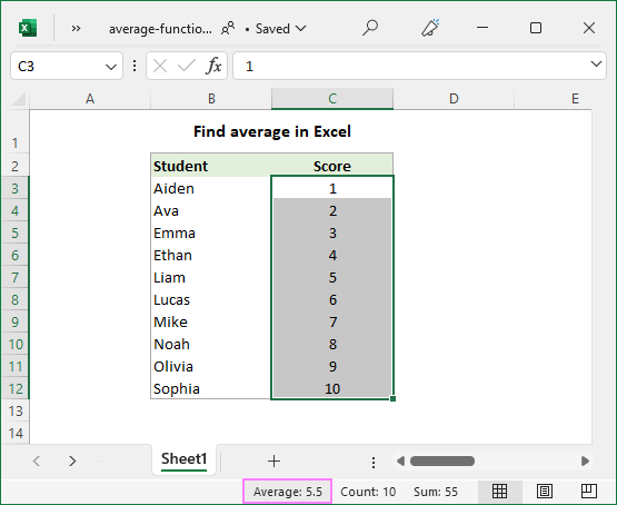
To quickly find an average without a formula, use Excel's status bar:
- Select the cells or ranges you want to average. For non-contiguous selections, use the Ctrl key.
- Look at the status bar at the bottom of the Excel window, which provides the essential information about the currently selected cells. One of the values that Excel calculates automatically is the average.
The result is shown in the image below:
If average is not displayed for your dataset, this article explains possible causes and solutions: Why Excel is not showing sum, average or count in the status bar.
How to calculate average manually
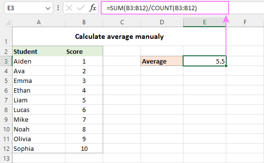
In math, to find the arithmetic mean of a list of numbers, you need to add up all the values, and then divide the sum by how many numbers there are in the list. In Excel, this can be done using the SUM and COUNT functions, respectively:
For the range of numbers below, the formula goes as follows:
=SUM(B3:B12)/COUNT(B3:B12)
As you can see, the result of the formula exactly matches the average value in the status bar.
In practice, you will hardly ever need to do a manual average in your worksheets. However, it may be useful to re-check the result of your average formula in case of doubt.
And now, let's take a look at how you can do average in Excel using the functions specially designed for the purpose.
AVERAGE function - calculate an average of numbers
You use the Excel AVERAGE function to get an average of all numbers in the specified cells or ranges.
Where number1, number2, … are numeric values for which you want to find the average. Up to 255 arguments can be included in a single formula. The arguments can be supplied as numbers, references, or named ranges.
AVERAGE is one of the most straightforward and easy-to-use functions in Excel.
To calculate an average of numbers, you can type them directly in a formula or supply the corresponding cell or range references.
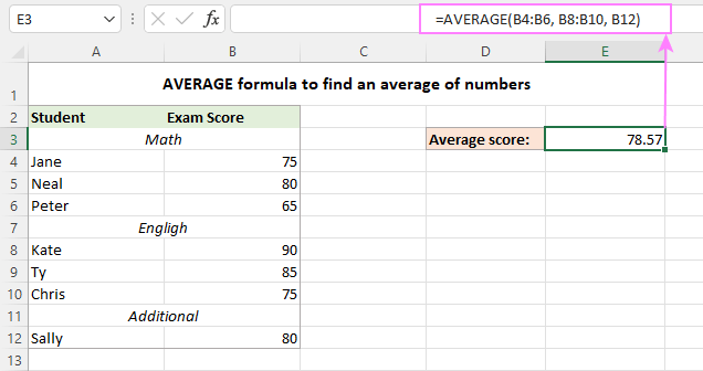
For example, to average 2 ranges and 1 individual cell below, the formula is:
=AVERAGE(B4:B6, B8:B10, B12)
Apart from numbers, the Excel AVERAGE function can find an average of other numeric values such as percentages and times.
Excel AVERAGE formula - usage notes
As you've just seen, using the AVERAGE function in Excel is easy. However, to get a correct result, you need to clearly understand what values are included in the average and what are ignored.
Included:
- Cells with zero values (0)
- Logical values TRUE and FALSE typed directly into the list of arguments. For example, the formula AVERAGE(TRUE, FALSE) returns 0.5, which is the mean of 1 and 0.
Ignored:
- Empty cells
- Text strings
- Cells containing Boolean values TRUE and FALSE
For more information, please see How to use AVERAGE function in Excel.
AVERAGEA function - average all non-blank cells
The Excel AVERAGEA function is similar to AVERAGE in that it calculates the arithmetic mean of the values in its arguments. The difference is that AVERAGEA includes all non-empty cells in a calculation, whether they contain numbers, text, logical values, or empty strings returned by other functions.
Where value1, value2, … are values, arrays, cell references or ranges that you want to average. The first argument is required, others (up to 255) are optional.
Excel AVERAGEA formula - usage notes
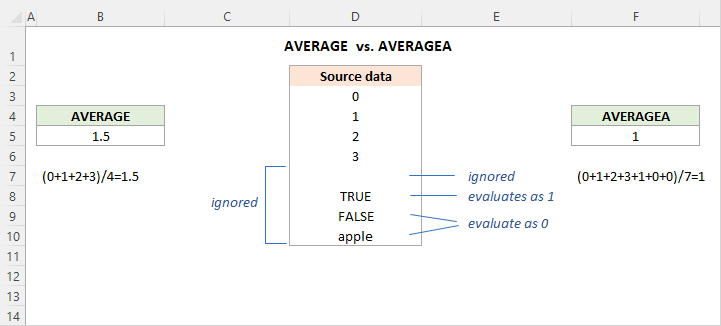
As mentioned above, the AVERAGEA function processes different value types such as numbers, text strings and logical values. And here's how they are evaluated:
Included:
- Text values evaluate as 0.
- Zero-length strings ("") evaluate as 0.
- Boolean value TRUE evaluates as 1 and FALSE as 0.
Ignored:
- Empty cells
For example, the below formula returns 1, which is the average of 2 and 0.
=AVERAGEA(2, FALSE)
The following formula returns 1.5, which is the average of 2 and 1.
=AVERAGEA(2, TRUE)
The image below demonstrates the AVERAGE and AVERAGEA formulas applied to the same list of values and different results they return:
AVERAGEIF function - get average with condition
To get the average of all cells in the specified range that meet a certain condition, use the AVERAGEIF function.
The AVERAGEIF function has the following arguments:
- Range (required) - the range of cells to test against a given criteria.
- Criteria (required) - the condition that should be met.
- Average_range (optional) - the cells to average. If omitted, then range is averaged.
The AVERAGEIF function is available in Excel 2007 - Excel 365. In earlier versions, you can build your own AVERAGE IF formula.
And now, let's see how you can use the Excel AVERAGEIF function to average cells based on the condition you specify.
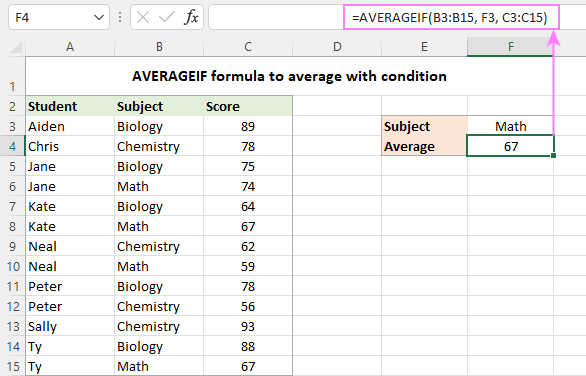
Suppose you have scores for different subjects in C3:C15 and you wish to find an average math score. This can be done with the following formula:
=AVERAGEIF(B3:B15, "math", C3:C15)
Instead of "hardcoding" the condition directly in a formula, you can type it in a separate cell (F3) and refer to that cell in the criteria:
=AVERAGEIF(B3:B15, F3, C3:C15)
For more formula examples, please see Excel AVERAGEIF function.
AVERAGEIFS function - average with multiple criteria
To do average with two or more conditions, use the plural counterpart of AVERAGEIF - the AVERAGEIFS function.
The function has the following syntax:
- Average_range (required) - the range to average.
- Criteria_range (required) - the range to be tested against criteria.
- Criteria (required) - the condition that determines which cells to average. It can be supplied in the form of a number, logical expression, text value, or cell reference.
1 to 127 criteria_range / criteria pairs can be supplied. The first pair is required, subsequent ones are optional.
In essence, you use AVERAGEIFS similarly to AVERAGEIF, except that more than one condition can be tested within a single formula.
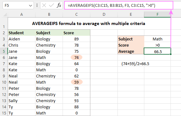
Supposing some students did not take tests in certain subjects and have zero scores. You aim to find an average score in a specific subject ignoring zeros.
To accomplish the task, you build an AVERAGEIFS formula with two criteria:
- Define the range to average (C3:C15).
- Specify the range to check against the 1st condition (B3:B15 - items).
- Express the 1st condition ("math" or F3 - the target item enclosed in quotation marks or reference to the cell containing the item).
- Specify the range to check against the 2nd condition (C3:C15 - scores).
- Express the 2nd condition (">0" - greater than zero).
By assembling the above components together, we get the following formula:
=AVERAGEIFS(C3:C15, B3:B15, "math", C3:C15, ">0")
Or
=AVERAGEIFS(C3:C15, B3:B15, F3, C3:C15, ">0")
The image below makes it clear that only two cells (C6 and C10) meet both conditions, and therefore only these cells are averaged.
For more information, check out Excel AVERAGEIFS function.
AVERAGEIF and AVERAGEIFS formulas - usage notes
Excel AVERAGEIF and AVERAGEIFS functions have much in common, in particular which values they calculate and which ignore:
- In the average range, empty cells, text values, logical values TRUE/FALSE are ignored.
- In criteria, empty cells are treated as zero values.
- The wildcard characters such as question mark (?) and asterisk (*) can be used in criteria for partial match.
- If no cell meets all of the specified criteria, a #DIV0! error occurs.
AVERAGEIF vs. AVERAGEIFS - differences
In terms of functionality, the most essential difference is that AVERAGEIF can only handle one condition while AVERAGEIFS one or more criteria. Also, there are a couple of technical differences related to average_range.
- With AVERAGEIF, average_range is the last and optional argument. In AVERAGEIFS formulas, it is the first and required argument.
- With AVERAGEIF, average_range does not necessarily have to be the same size as range because the actual cells to be averaged are determined by the size of the range argument - the upper left cell of average_range is taken as the starting point, and as many cells are averaged as included in the range argument. AVERAGEIFS requires each criteria_range to be of the same size and shape as average_range, otherwise a #VALUE! error occurs.
AVERAGE IF OR formula in Excel
Since the Excel AVERAGEIFS function always works with the AND logic (all criteria must be TRUE), you will have to construct your own formula to average cells with the OR logic (any single criterion must be TRUE).
Here's the generic formula to average if cell is X or Y.
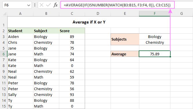
Now, let's see how it works in practice. In the table below, suppose you want to find an average score of two subjects, Biology and Chemistry, which are input in cells F3 and F4. This can be done with the following array formula:
=AVERAGE(IF(ISNUMBER(MATCH(B3:B15, {"biology", "chemistry"}, 0)), C3:C15))
Translated into a human language, the formula says: average cells in C3:C15 if a corresponding cell in B3:B15 is either "Biology" or "Chemistry".
Instead of the hardcoded criteria, you can use a range reference (F3:F4 in our case):
=AVERAGE(IF(ISNUMBER(MATCH(B3:B15, F3:F4, 0)), C3:C15))
For the formula to work correctly, please remember to press Ctrl + Shift + Enter in Excel 2019 and lower. In dynamic array Excel (365 and 2021), a regular Enter hit will suffice:
How this formula works:
For our curious and thoughtful readers who want not only to use a formula but understand what they are doing, here's a detailed explanation of the logic.
At the core of the formula, the IF function determines which values in the source range match any of the specified criteria and passes those values to the AVERAGE function. Here's how:
The MATCH function uses the subject names in B3:B15 as the lookup values and compares each of those values against the lookup array in F3:F4 (our target subjects). The 3rd argument (match_type) is set to 0 to look for exact match:
MATCH(B3:B15, F3:F4, 0)
When a match is found, MATCH returns its relative position in the lookup array, otherwise an #N/A error:
{1;2;1;#N/A;1;#N/A;2;#N/A;1;2;2;1;#N/A}
The ISNUMBER function converts numbers to TRUE and errors to FALSE:
{TRUE;TRUE;TRUE;FALSE;TRUE;FALSE;TRUE;FALSE;TRUE;TRUE;TRUE;TRUE;FALSE}
This array goes to the logical test of IF. In the full form, the logical test should be written like this:
IF(ISNUMBER(MATCH(B3:B15, F3:F4, 0))=TRUE
For the sake of brevity, we omit the =TRUE part because it's implied.
By setting the value_if_true argument to C3:C15, you tell the IF function to replace TRUE's with the actual values from C3:C15:
{89;78;75;FALSE;64;FALSE;62;FALSE;78;56;93;88;FALSE}
This final array is handed over to the AVERAGE function that calculates an arithmetic mean of numbers ignoring logical values.
How to round average in Excel
When calculating an average in Excel, the result is often a number with multiple decimal places. In case you want to display fewer decimal digits or round an average to an integer, use one of the following solutions.
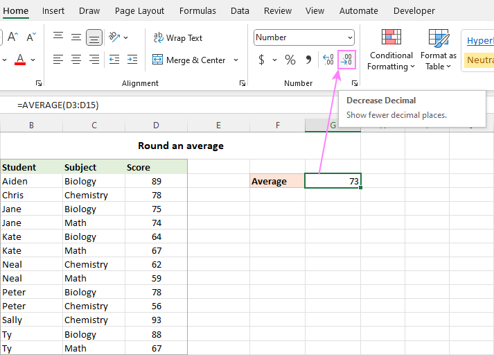
Decrease Decimal option
To round only the displayed average without changing the underlying value, the fastest way is to utilize the Decrease Decimal command on the Home tab, in the Number group:
Format Cells dialog box
The number of decimal places can also be specified in the Format Cells dialog box. To have it done, select the formula cell and press Ctrl + 1 to open the Format Cells dialog. Then, switch to the Number tab, and type the number of places you want to show in the Decimal places box.
Like the previous method, this changes only the display format. When referring to the average cell in other formulas, the original non-rounded value will be used in all calculations.

For full details, please see Round numbers by changing cell format.
Round an average with a formula
To round the calculated value itself, wrap your average formula in one of the Excel rounding functions.
In most situations, you'd use the ROUND function that follows the general math rules for rounding. In the 1st argument (number), nest the AVERAGE, AVERAGEIF or AVERAGEIFS function. In the 2nd argument (num_digits), specify the number of decimal places to round the average to.
For example, to round off an average to the nearest integer, the formula is:
=ROUND(AVERAGE(B3:B15), 0)
To round an average to one decimal place, this is the formula to use:
=ROUND(AVERAGE(B3:B15), 1)
To round an average to two decimal places, this one will work:
=ROUND(AVERAGE(B3:B15), 2)

That is how you can do average in Excel. Below there are links to the related tutorials that discuss more specific cases of average, hope you will find them helpful. Thank you for reading!
Practice workbook for download
Calculate average in Excel - examples (.xlsx file)
 by
by
52 comments
I'm trying to build this formula: =(C6-(AVERAGE($C$4:$C6))/AVERAGE($C$4:$C6))
but the result is wrong. I tried to find out where it is wrong but I failed.
any help will be much appreciated.
Hi! If the cells are empty, the formula will return the error #DIV/0! because you cannot divide by 0. Also, (AVERAGE($C$4:$C6))/AVERAGE($C$4:$C6) always equals 1 if there is at least one value. Therefore, you can write =C6-1
Also read more: How to divide in Excel and handle #DIV/0! error
Dear Sir,
I really appreciate that you are supporting to the students.
Here i need a formula to get the value as
we have a table containing x ordinate and y ordinate value and now formula we need is the value (x,y) =?
Hi! With these two numbers, you can get a cell reference using the ADDRESS function. To get a value from a cell on this reference, you can use the INDIRECT function.
For example:
=INDIRECT(ADDRESS(5,2))
You can also get the value of a cell that is offset by x number of columns and y number of rows relative to the starting cell. Use OFFSET function:
=OFFSET(D7,5,2)
Thank you for our column.
my question is I want the average temperature for the past 10 days.
The temperatures are in column A rows 2 through 11
The average is calculated in Column B Row 1
On day 11 I want to add the current temperature, preferably in Column A row 2 using INSERT and moving the old data down 1 row.
Using a $ to designate absolute cells does not work, when I use INSERT the formula changes to match the old data.
For example before insert the formula is: =Average(A$2:A$11 but after inserting a cell in A2 and selecting "shift cells down" the formula changes to =Average(A$3:A$12)
Thank you for any assistance
Hello! Convert the range A1:A11 into a table. Read how to do it here: Excel table: end-to-end tutorial with examples. Use structured references in the formula for calculating the average value. For example:
=AVERAGE(Table1[temp])
Then when you insert row 2, a row will be added to the table and the formula will not change.
Thank you very much for your assistance!
Hi, I'm trying to get the averages of stats after each basketball game in a season; i.e., free throws, rebounds, etc. I have manually entered the first four 'average' formulas, but wanted to have it done automatically with a formula, so i didn't have to add each new game to the formula manually. Here is a portion of my spreadsheet:
Rebounds Avg Rebounds
3 3
6 4.5
3 4
4 * this column is where I want the formula to automatically calculate so I don't have to manually update the formula after every game
Hi! Maybe this article will be helpful: How to copy formula in Excel with or without changing references.
Can I use AVERAGEIFS to get the average of two AVERAGEIFS calculations?
Example: I want to calculate the average of both of these ranges located on two separate sheets
=averageifs('2022 Survey Data'!D:D, '2022 Survey Data'!L:L, ">04/01/2022",'2022 Survey Data'!L:L,"<05/01/2022", '2022 Survey Data'!D:D, "")
and
=averageifs('2022 Zoom Data'!D:D, '2022 Zoom Data'!L:L, ">04/01/2022",'2022 Zoom Data'!L:L,"<05/01/2022", '2022 Zoom Data'!D:D, "")
Hello!
I can't check the formula that contains unique references to your workbook worksheets. Each of your formulas returns a value to the cell in which it is written. Calculate the average of these two cells using the AVERAGE function.
Or you can use these formulas as arguments for the AVERAGE function.
=AVERAGE(averageifs(‘2022 Survey Data’!D:D, ‘2022 Survey Data’!L:L, “>04/01/2022″,’2022 Survey Data’!L:L,”<05/01/2022", '2022 Survey Data'!D:D, "”), averageifs(‘2022 Zoom Data’!D:D, ‘2022 Zoom Data’!L:L, “>04/01/2022″,’2022 Zoom Data’!L:L,”<05/01/2022", '2022 Zoom Data'!D:D, "”))
Dear Svetlana
I need to easy average fonction. I have table for sold products KG and the rate. I need to average rate of the each products. You can see below a small table but my real table is huge.
Product - KG - Rate
A - 120 - 1,50
B - 85 - 3,40
C - 90 - 2,75
A - 110 - 1,53
A - 113 - 1,48
C - 85 - 2,68
Hello!
If you want to calculate the average for a product, use the AVERAGEIF function as described in this article. If you need to calculate a weighted average, use this guide.
Hi, fab article. Is there any way to do an AverageIF on selected cells within a row. E.g. the data to average is not continuous but has gaps to avoid?
Many thanks
Hi,
If by gaps you mean empty cells, then this case is described in detail in the manual above. Use AVERAGEIFS. Also remember that there can only be one counting range for the AVERAGEIF function.
I need to average every 5th cell in a row for a workbook that will be recording daily input, it needs to extend on for continued use. I'm using this format and from what I can tell it should work, but averages are puling numbers from every cell not just every 5th cell.
=Average(IF(MOD(COLUMN(G3:AA3),5)=0,G3:AA3))
Yes, I am pressing Shift+Ctrl+Enter.
Please Help
Hello!
If I understand your task correctly, the following formula should work for you:
=Average(IF(MOD(COLUMN(G3:AA3),5)=1,G3:AA3))
I hope it’ll be helpful.
Lol, guess i should have checks to see if anyone was answering all the questions before I asked mine.
please sir i need a formulas basic because i learned first time but i want to learned excel formula
Hello Abbasi,
Hopefully, you will find this tutorial helpful:
Basic Excel formulas & functions with examples
Dear Svetlana,
Thks for your update.
I learned some shortcuts. I would like to learn the Macro as well. I hope u can suggest better way to learn the Macro.
Kind Regards,
Ram.
Hi Ramaraj,
We have a couple of tutorials on Excel macros. Please check out these ones:
How to insert and run VBA code in Excel - tutorial for beginners
Tutorial with Excel examples about Macros
Now any input for Max (IF) formula:
=MAX(IF('sheet1'!A:A=J4,'sheet1'!T:T))
In above formula, it consider the Max in column T, by returning name "Truck" in column A. // J4=Truck
Now, if I want to add that dates frame (formula part), how should I go through:
'sheet1'!B:B,">="&P2,'sheet1'!B:B,"<="&P3
P2= Start date
P3= End date
Thanks in advance for your input.
Hello,
Please try the following formula:
=MAXIFS('sheet1'!T:T, 'sheet1'!A:A, J4, 'sheet1'!B:B, ">="&P2, 'sheet1'!B:B, "<="&P3)
Hope it will help you.
I have a formula which is like this
=AVERAGEIF('sheet1'!A:A,"Truck",'sheet1'!V:V)
which is take the average of all data in column V (sheet1) based on all info related to the Truck in column A.
Now, I want this formula to read the same information but by consider a range of dates in between 1st of October to 15th (I have dates in Column B in the same sheet1).
The formula I created for the second part is like this, but can not merge it to the first part:
'sheet1'!B:B,">="&P2,'sheet1'!B:B,"<="&P3
P2= Start date
P3= End date
Hello,
Please try the following formula:
=AVERAGEIFS('sheet1'V:V,'sheet1'A:A,"Truck",'sheet1'B:B," > ="&P2,'sheet1'B:B," < ="&P3)
Hope it will help you.
Hello and Thanks for your feedback,
It apparently do something, but gave me #DIV/0! error, it should give me a 2.53.
Any input?
Hello,
Please check the following:
1 The ">=" и "<=" conditions in the formula don't contain any spaces.
2 The P2 and P3 cells in your table contain dates.
3 The 'sheet1'!V:V range for calculating an average value is not empty or doesn’t contain text values.
4 The 'sheet1'!A:A and 'sheet1'!B:B ranges with selection criteria are not empty as well.
Can someone help me figure out what is wrong with this function:
{=AVERAGE(IF(CementByRegion!B3:B42,Sheet1!J20,CementByRegion!C3:G42))}
J20="Text" that shows up in column "B". I'm trying to do an average of data in more than one column.
Hello,
I believe this will do :)
=AVERAGEIF(CementByRegion!B3:B42,"="&Sheet1!J20, CementByRegion!C3:G42)
Dear Svetlana & Community,
thanks for the great tutorials.
I am trying to average a selection of non-continous columns, all titled "kcal in".
I have set the columns DF2:XA2 as the range, which is the title column. "kcal in" is the crietria and DF4:$XA$435 is the average of all kcal in in the DF4 row. I can drag the formula down to obtain the average for rows DF5 etc.
=AVERAGEIF($DF$2:$XA$2, "kcal in", DF4:$XA$435)
This works well, however, I am trying to exclude any 0 values in row DF4 from the average and I am not sure where to put this criterion.
Many thanks in advance for your help
Found the answer here myself :)
=AVERAGEIFS(DF6:XA6,$DF$2:$XA$2,"kcal in",DF6:XA6,">0")
Adapted from your explanation
Average_range is DF6:XA6 (the row you want to average if both conditions are met);
Criteria_range1 is $DF$2:$XA$2 (the head column, range fixed with dollar sign) and criteria1 is "kcal in"(allowing to average non-continuous columns)
Criteria_range2 is DF6:XA6 (the row you want to average) and criteria2 is ">0". (values of 0 are excluded)
Thanks for the great site, finally my mind can rest :D
Hi , i am trying to find an average based on criteria :
Example 1 : A1 = 3, E1=2 , J1 = 10, My answer will be A1+E1+J1/3 = 5.
Example 2 A1 = 3, E1 = 3, J1 = -, My answer will be A1+E1+J1/3 = 3.
Example 3 A1 = -, E1 = -, J1 = -, My answer should be A1+E1+J1/3 = 0.
Example 1 and 2 is Ok, Where as in example 3 am getting error #DIV/0! instead of this i need 0 in the box.
Thanks in advance
Hi,
please note that empty cells are ignored by AVERAGE function.
Try entering zero (0) in the cells, if you want zero to return.
Hope it helps!
hi, i need to get the average of below data but it seems like im having problem, just one category from type is getting. THANKS SO MUCH IN ADVANCE:)
here's my formula: =AVERAGEIFS(D:D,B:B,"prior20",C:C,"cavite",E:E,{"crtfixed","crtvoice","rbg-crt"})
A B C D
date area ave type
prior20 cavite 10 crtfixed
prior20 cebu 9 crtvoice
prior20 makati 8 rbg-crt
prior20 cavite 7 crtfixed
prior20 cebu 6 crtfixed
prior20 makati 5 crtvoice
prior20 cavite 4 rbg-crt
prior20 cebu 3 crtfixed
beyond luzon 2 crtfixed
prior20 makati 5 crtvoice
prior20 cavite 4 rbg-crt
prior20 cebu 3 crtfixed
Hi Mitch,
try this formula:
=SUM(SUMIFS(D:D,B:B,"prior20",C:C,"cavite",E:E,{"crtfixed","crtvoice","rbg-crt"}))/SUM(COUNTIFS(B:B,"prior20",C:C,"cavite",E:E,{"crtfixed","crtvoice","rbg-crt"}))
I want to auto calculate average of every five cells of a column to another column. I have daily rainfall data for 30 years but I want average of every 5 days of each year.
Hi Jide,
It sounds like you want to calculate a moving average. Please the examples here:
https://www.ablebits.com/office-addins-blog/moving-average-excel/
I am using an AVERAGEIF formula using ranges that have been rounded up and down. When I evaluate my formula the range changes from say 9.0 to 8.999999999 which then means the formula produces a #DIV/0! value.
Can you help with sorting this out please?
Sorry, that should have read AVERAGEIFS
Cheers
Hi, Could you please tell me how can i calculate average excluding blank boxes in excel?
Hi!
By default, the Excel Average function excludes blank cells from an average, though cells with zero values are included.
Hi,
I want to do average of the values using averageif formulae, these values contain 0 also but I want to exclude these Os from the formula.
Please suggest which formula to use.
Hello Avnish,
Use the AVERAGEIFS function and include "is not equal to 0" ("<>"&0) as one of the criteria.