Excel substring functions to extract text from cell

The tutorial shows how to use the Substring functions in Excel to extract text from a cell, get a substring before or after a specified character, find cells containing part of a string, and more.

Before we start discussing different techniques to manipulate substrings in Excel, let's just take a moment to define the term so that we can begin on the same page. So, what is a substring? Simply, it's part of a text entry. For example, if you type something like "AA-111" in a cell, you'd call it an alphanumeric string, and any part of the string, say "AA", would be a substring.

Although there is no such thing as Substring function in Excel, there exist three Text functions (LEFT, RIGHT, and MID) to extract a substring of a given length. Also, there are FIND and SEARCH functions to get a substring before or after a specific character. And, there are a handful of other functions to perform more complex operations such as extracting numbers from a string, replacing one substring with another, looking up partial text match, etc. Below you will find formula examples to do all this and a lot more.

How to extract substring of a certain length

Microsoft Excel provides three different functions to extract text of a specified length from a cell. Depending on where you want to start extraction, use one of these formulas:

LEFT function - to extract a substring from the left.
RIGHT function - to extract text from the right.
MID function - to extract a substring from the middle of a text string, starting at the point you specify.

As is the case with other formulas, Excel substring functions are best to learn from an example, so let's look at a few ones.

Extract substring from start of string (LEFT)

To extract text from the left of a string, you use the Excel LEFT function:

LEFT(text, [num_chars])

Where text is the address of the cell containing the source string, and num_chars is the number of characters you want to extract.

For example, to get the first 4 characters from the beginning of a text string, use this formula:

=LEFT(A2,4)
LEFT formula to extract a substring from the start of a string

Get substring from end of string (RIGHT)

To get a substring from the right part of a text string, go with the Excel RIGHT function:

RIGHT(text, [num_chars])

For instance, to get the last 4 characters from the end of a string, use this formula:

=RIGHT(A2,4)
RIGHT formula to extract a substring from the end of a string

Extract text from middle of string (MID)

If you are looking to extract a substring starting in the middle of a string, at the position you specify, then MID is the function you can rely on.

Compared to the other two Text functions, MID has a slightly different syntax:

MID(text, start_num, num_chars)

Aside from text (the original text string) and num_chars (the number of characters to extract), you also indicate start_num (the starting point).

In our sample data set, to get three characters from the middle of a string beginning with the 6th character, you use the following formula:

=MID(A2,6,3)
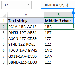
MID formula to extract text from the middle of a string

Tip. The output of the Right, Left and Mid formulas is always text, even when you are extracting a number from a text string. If you want to operate on the result as a number, then wrap your formula in the VALUE function like this:

=VALUE(MID(A2,6,3))

Extract substring before or after a given character

As shown in the above examples, the Left, Right and Mid functions cope nicely with uniform strings. When you are dealing with text strings of variable length, more complex manipulations shall be needed.

Note. In all of the below examples, we will be using the case-insensitive SEARCH function to get the position of a character. If you want a case-sensitive formula, use the FIND function instead.

How to extract text before a specific character

To get a substring preceding a given character, two things are to be done: first, you determine the position of the character of interest, and then you pull all characters before it. More precisely, you use the SEARCH function to find the position of the character, and subtract 1 from the result, because you don't want to include the character itself in the output. And then, you send the returned number directly to the num_chars argument of the LEFT function:

LEFT(cell, SEARCH("char", cell)-1)

For example, to extract a substring before the hyphen character (-) from cell A2, use this formula:

=LEFT(A2, SEARCH("-",A2)-1)

No matter how many characters your Excel string contains, the formula only extracts text before the first hyphen:
Extracting text before a specific character

How to extract text after character

To get text following a specific character, you use a slightly different approach: get the position of the character with either SEARCH or FIND, subtract that number from the total string length returned by the LEN function, and extract that many characters from the end of the string.

RIGHT(cell,LEN(cell)-SEARCH("char", cell))

In our example, we'd use the following formula to extract a substring after the first hyphen:

=RIGHT(A2,LEN(A2)-SEARCH("-",A2))
Extracting text after a specific character

How to extract text between two instances of a character

To get a substring between two occurrences of a certain character, use the following generic formula:

MID(cell, SEARCH("char", cell)+1, SEARCH ("char", cell, SEARCH ("char", cell)+1) - SEARCH ("char", cell)-1)

The first two arguments of this MID formula are crystal clear:

Text is the cell containing the original text string.

Start_num (starting point) - a simple SEARCH formula returns the position of the desired character, to which you add 1 because you want to start extraction with the next character.

Num_chars (number of chars to extract) is the trickiest part:

First, you work out the position of the second occurrence of the character by nesting one Search function within another.
After that, you subtract the position of the 1st occurrence from the position of the 2nd occurrence, and subtract 1 from the result since you don't want to include the delimiter character in the resulting substring.

For example, to extract text surrounded by two hyphens, you'd use this formula:

=MID(A2, SEARCH("-",A2) + 1, SEARCH("-",A2,SEARCH("-",A2)+1) - SEARCH("-",A2) - 1)

The screenshot below shows the result:
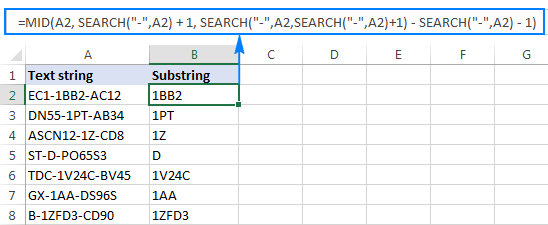
Extracting text between two hyphens

If you are looking to extract text between 2^nd and 3^rd or 3^nd and 4^th occurrences of the same character, you can use a more compact SEARCH SUBSTITUTE combination to get the character's position, as explained in How to find Nth occurrence of a character in a string:

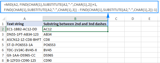
FIND(CHAR(1),SUBSTITUTE(cell,character,CHAR(1),Nth occurrence))

In our case, we could extract a substring between the 2nd and 3rd hyphens with the following formula:

=MID(A2, FIND(CHAR(1),SUBSTITUTE(A2,"-",CHAR(1),2))+1, FIND(CHAR(1),SUBSTITUTE(A2,"-",CHAR(1),3)) - FIND(CHAR(1),SUBSTITUTE(A2,"-",CHAR(1),2))-1)
Extracting a substring between the 2nd and 3rd hyphens

How to find substring in Excel

In situations when you don't want to extract a substring and only want to find cells containing it, you use the SEARCH or FIND function as shown in the above examples, but perform the search within the ISNUMBER function. If a cell contains the substring, the Search function returns the position of the first character, and as long as ISNUMBER gets any number, it returns TRUE. If the substring is not found, the search results in an error, forcing ISNUMBER to return FALSE.

ISNUMBER(SEARCH("substring", cell))

Supposing, you have a list of British postcodes in column A and you want to find those that contain the substring "1ZZ". To have it done, use this formula:

=ISNUMBER(SEARCH("1zz", A2))

The results will look something similar to this:
Finding cells that contain a specific substring

If you'd like to return your own message instead of the logical values of TRUE and FALSE, nest the above formula into the IF function:

=IF(ISNUMBER(SEARCH("1zz", A2)), "Yes", "")

If a cell contains the substring, the formula returns "Yes", an empty string ("") otherwise:
Formula to identify cells that contain a certain substring

As you may remember, the Excel SEARCH function is case-insensitive, so you use it when the character case does not matter. To get your formula to distinguish the uppercase and lowercase characters, opt for the case-sensitive FIND function.

For more information on how to find text and numbers in Excel, please see If cell contains formula examples.

How to extract text from cell with Ultimate Suite for Excel

As you have just seen, Microsoft Excel provides an array of different functions to work with text strings. In case you are unsure which function is best suited for your needs, commit the job to our Ultimate Suite for Excel. With these tools in your Excel's arsenal, you just go to Ablebits Data tab > Text group, and click Extract:
Extract Text tool in Excel

Now, you select the source cells, and whatever complex strings they contain, a substring extraction boils down to these two simple actions:

Specify how many characters you want to get from the start, end or middle of the string; or choose to extract all text before or after a given character.
Click Insert Results. Done!

For example, to pull the domain names from the list of email addresses, you select the All after text radio button and type @ in the box next to it. To extract the user names, you select the All before text radio button, as shown in the screenshot below.
Define the substring you want to extract.

And you will get the following results in a moment:
Parts of email addresses are extracted in separate columns.

Apart from speed and simplicity, the Extract Text tool has extra value - it will help you learn Excel formulas in general and substring functions in particular. How? By selecting the Insert as formula checkbox at the bottom of the pane, you ensure that the results are output as formulas, not values.

In this example, if you select cells B2 and C2, you will see the following formulas, respectively:

To extract username:
=IFERROR(LEFT(A2,SEARCH("@",A2)-1),"")
To extract domain:
=IFERROR(RIGHT(A2, LEN(A2)- SEARCH("@",A2) - LEN("@") + 1),"")

How much time would it take you to figure out these formulas on your own? ;)

Since the results are formulas, the extracted substrings will update automatically as soon as any changes are made to the original strings. When new entries are added to your data set, you can copy the formulas to other cells as usual, without having to run the Extract Text tool anew.

If you are curious to try this as well as many other useful features included with Ultimate Suite for Excel, you are welcome to download evaluation version.

More formulas for substrings in Excel

In this tutorial, we have demonstrated some classic Excel formulas to extract text from string. As you understand, there can be almost infinite variations of these basic scenarios. Below you will find a few more formula examples where the Text functions come in handy.

How to extract number from string in Excel - formula examples to get a number from various text strings.
How to extract Nth word from a text string - how to use MID in combination with 4 other functions to get any Nth word from a cell.
How to extract a word containing a certain substring - one more non-trivial MID formula that pulls a word containing a specific character(s) from anywhere in the source string.
How to extract text between parentheses - using this approach, you can get a substring between any two characters you specify.
How to Lookup partial string match - how to use an Excel substring function (LEFT, RIGHT or MID) in combination with Vlookup to retrieve values based on partial match.
How to replace one substring with another - a formula to find and replace a certain character or substring within the text string.
How to count cells containing a substring - how to use the COUNTIF function with wildcard characters to count cells containing specific text, i.e. count with partial match.
Excel RegEx to extract subsrtings - how to extract text and special characters using regular expressions.
Extract text between two characters - how to find and extract text from string between two characters or words in Excel and Google Sheets.
Custom function to extract word from string - how to get first, second, last or Nth words from text without lengthy and complex formulas.

Available downloads

Excel substring functions - practice workbook (.xlsx file)
Ultimate Suite - trial version (.exe file)

Latest comments

Cameron Searle
2025-09-08

Good afternoon,

I have one column, full of rows of text and I need to display in a new column a particular text that relates to a particular word. I tried the ifcount but can only do it 64 times.

Here's an example.

Row 1 contain: The company placed a dog in a kennel
Row 2 contain: The department store has a cat in a litter box
Row 3 contain: Litter boxes are bought in Australia

For row 1 I want the word "Pet" bough back and row 3 "House" bought back.

This is how I would do it. =if(countif(A1,"*dog*"),"Pet",if(countif(A2,"*cat*"),"Pet",if(count(A3,"*litter*"),"House"," ")))

Is there a better way because I have 2,000 rows of data.
1. Alexander Trifuntov (Ablebits Team)
  2025-09-08
  
  Hello Cameron!
  If you want to use multiple conditions to determine whether text matches, try the IFS function. You can find the examples and detailed instructions here: Use the Excel IFS function instead of nested IF.
Ryan P
2025-07-15

I need to pull out the number with hyphen in each cell. Some cells have more hyphenated numbers than others (some have 1, others have many). Each number has a description with it that I don't want to keep. The common text is the hyphen with 2 numbers in front and 3 behind. Is there a way to extract the numbers into a cell leaving the letters behind?

2 examples:

05-100 METAL FABRICATION, 05-150 STRUCTURAL STEEL ERECTION, 05-500 MISC METAL FABRICATION
--- I'd like the list in the cell to read 05-100 ; 05-150 ; 05-500 which adds a space, semi-colon, and space between each number group.

07-302 SHINGLE ROOFING, 07-402 SIDING & SOFFIT, 07-410 METAL ROOFING, 07-500 BUILT UP -RUBBER ROOF (TPO), 07-600 SHEETMETAL - FLASHING
--- I'd like the list in the cell to read 07-302 ; 07-402 ; 07-410 ; 07-500 ; 07-600

Thanks,
Ryan
1. Alexander Trifuntov (Ablebits Team)
  2025-07-16
  
  Hello Ryan!
  You can extract all of the pattern matching from text using regular expressions. For detailed instructions, see here: How to extract substrings in Excel using regular expressions (Regex). The formula might look like this:
  
  =TEXTJOIN(", ",TRUE, RegExpExtract(A1, "\d{2}[-\. ]?\d{3}"))
  
  I recommend paying attention to the Regex tool. You can find, extract, compare, delete, or replace strings that match the regular expression pattern you enter. You don't need to install any VBA code. It is available as a part of our Ultimate Suite for Excel that you can install in a trial mode and check how it works for free.
  1. Ryan P
    2025-07-16
    
    Thank you. I'll give it a try.
Rajawali
2025-06-10

Dear Sir,

Could you help me to solve the following?

I'd like to extract specific text with several option of criteria which is started with "SA-" or "WO-" "PO-", Currently I can only solve it for 1 criteria only, using the following formula:

=TRIM(LEFT(SUBSTITUTE(MID(I7865;FIND("SA-";I7865);LEN(I7865));" ";REPT(" ";100));100))

Thanks in advance,
Akbar
1. Alexander Trifuntov (Ablebits Team)
  2025-06-10
  
  Hi! To extract a text string from a cell after one of several characters, use an array of values in FIND function. Replace search errors with emptiness using IFERROR function. Then combine results into a text string, ignoring empty values, using TEXTJOIN function. For example:
  
  =TEXTJOIN("",TRUE, IFERROR(TRIM(LEFT(SUBSTITUTE(MID(A1,FIND({"SA-","WO-"},A1),LEN(A1))," ",REPT(" ",100)),100)),""))
marlon
2025-05-20

How can I get the sum of two cells if letters and numbers are in same cell?
Example: B3 Bernardino 21000 and B4 Ravida 14253
1. Alexander Trifuntov (Ablebits Team)
  2025-05-21
  
  Hi! To find sum of numbers, you need to extract those numbers from text and convert them to normal numbers. You can use these instructions: Extract number from the right of a string. For example:
  
  =IFERROR(RIGHT(B3, LEN(B3) - MAX(IF(ISNUMBER(MID(B3, ROW(INDIRECT("1:"&LEN(B3))), 1) *1)=FALSE, ROW(INDIRECT("1:"&LEN(B3))), 0))) +0, "") + IFERROR(RIGHT(B4, LEN(B4) - MAX(IF(ISNUMBER(MID(B4, ROW(INDIRECT("1:"&LEN(B4))), 1) *1)=FALSE, ROW(INDIRECT("1:"&LEN(B4))), 0))) +0, "")
Olga
2025-03-27

Hi, how to extract only latin letters from a string with all kinds of symbols? Thanks.
1. Alexander Trifuntov (Ablebits Team)
  2025-03-27
  
  Hello Olga!
  Use MID function to sequentially extract all characters from the text. If this character is found with FIND function in the list of allowed characters, merge it into a new text string with TEXTJOIN function. You can use this formula:
  
  =TEXTJOIN("", TRUE, IF(ISNUMBER(FIND(MID(A1, ROW(INDIRECT("1:"&LEN(A1))), 1), "ABCDEFGHIJKLMNOPQRSTUVWXYZabcdefghijklmnopqrstuvwxyz")), MID(A1, ROW(INDIRECT("1:"&LEN(A1))), 1), ""))
Zoe McShane
2025-01-10

Hi I have used used =LEFT(A4,SEARCH("-",A4)-1) formula to take the first 2 words from my A4 cell which is a string of text and numbers but I want to turn the output to the words seperated is this possible?

i.e. A4 cell: john.doe-250110-12345
using above function B4 cell is john.doe

what I want is John Doe

Many thanks in advance :)
1. Alexander Trifuntov (Ablebits Team)
  2025-01-13
  
  Hello Zoe!
  Extract the first two words from the text using the “-” separator. You can find the examples and detailed instructions here: How to extract word from string in Excel: first, last, Nth, and more.
  From this text string, extract the first and last word. The formulas might look like this:
  
  =LEFT(LEFT(A1,SEARCH("-",A1)-1), SEARCH(".",LEFT(A1,SEARCH("-",A1)-1))-1)
  =MID(LEFT(A1,SEARCH("-",A1)-1), SEARCH(".",LEFT(A1,SEARCH("-",A1)-1))+1,20)
  
  Maybe this article also will help: Capitalize first letter in Excel cells.
Abhineet
2024-12-26

Hi, I would like to extract only text from the number.
Ex- Kevin Thomas78455. How do I do that? Please help!
1. Alexander Trifuntov (Ablebits Team)
  2024-12-27
  
  Hi! We have a special tutorial on this. Please see: Extract number from text string.
  Please check the formulas below; they should work for you.
  
  =SUMPRODUCT(MID(0&A1, LARGE(INDEX(ISNUMBER(--MID(A1, ROW(INDIRECT("1:"&LEN(A1))), 1)) * ROW(INDIRECT("1:"&LEN(A1))), 0), ROW(INDIRECT("1:"&LEN(A1))))+1, 1) * 10^ROW(INDIRECT("1:"&LEN(A1)))/10)
  or
  =CONCAT(IF(ISNUMBER(--MID(A1,ROW($1:$50),1)),MID(A1,ROW($1:$50),1),""))
Kim
2024-11-10

P10-ABC-3234
P10-ABC-3234-1234

I would like to extract last numbers after "-" from the right

=right(A2,len(A2)-Search("-",A2) would give me ABC-3234, should i have to use 2 times same formula?

would would the formula please.
1. Alexander Trifuntov (Ablebits Team)
  2024-11-11
  
  Hello Kim!
  If I understand your task correctly, the following tutorial should help: How to extract last word in Excel.
  
  =TRIM(RIGHT(SUBSTITUTE(A2, "-", REPT(" ", LEN(A2))), LEN(A2)))
  
  You can also use in Excel for Microsoft 365 the TEXTAFTER function. See more: Get text after last occurrence of delimiter.
  
  =TEXTAFTER(A2, "-", -1)
Chloe
2024-10-01

How do i extrace only lower case characters in a string of excel?
1. Alexander Trifuntov (Ablebits Team)
  2024-10-01
  
  Hello Chloe!
  Extract each character from the text individually using MID function.
  Convert them to lower case using LOWER function.
  Compare the converted lower case character with the original character using EXACT function to determine an exact match.
  If the characters are the same, add the character to a new text string created with TEXTJOIN function as described here.
  The formula might look something like the following:
  
  =TEXTJOIN("",TRUE, IF(EXACT(MID(A1,ROW(INDIRECT("1:"&LEN(A1))),1), LOWER(MID(A1,ROW(INDIRECT("1:"&LEN(A1))),1))), MID(A1,ROW(INDIRECT("1:"&LEN(A1))),1),""))
Isis Jhanine
2023-05-31

HI! i need a super big help. I'd love to have your knowledge and expertise to find a solution to this:

i have two columns with information (text) that is not coming in the same order EX:

Column A: Finance Service Account; HR Business Partner; Client Account
Column B: Client Account; Finance Service Account

I am ok with the ones which are repeated, i want a formula to find the differences between the two columns and throw the HR Business Partner as a result. your help would be very much appreciated. thank you!
1. Alexander Trifuntov (Ablebits Team)
  2023-06-01
  
  Hi! If I understand your task correctly, the following formula should work for you:
  
  =IF(CONCAT(CHOOSECOLS(TEXTSPLIT(A1,";"),3,1)) = CONCAT(TEXTSPLIT(B1,";")), CHOOSECOLS(TEXTSPLIT(A1,";"),2),"")
  
  Use the TEXTSPLIT function to split the text by separators. Use the CHOOSECOLS function to get the desired parts of the text. Combine these parts with the CONCAT function and compare them.
Maris
2023-03-29

Hi!

I have a cell with multiplication formula. for example c2 is "=3,2*2,6". I want to take those 3,2 to d2, and 2,6 to e2.

Sorry for my english!
1. Alexander Trifuntov (Ablebits Team)
  2023-03-29
  
  Hi!
  If your formula is written as text, use substring functions to extract numbers from text.
  
  =--LEFT(C2,SEARCH("~*",C2)-1)
  =--MID(C2,SEARCH("~*",C2)+1,10)
  
  If a formula is written in cell C2, use FORMULATEXT to get formula text.
  =--LEFT(FORMULATEXT(C2),SEARCH("~*",FORMULATEXT(C2))-1)
  
  I hope my advice will help you solve your task.
Carl Thomas Byerley
2023-03-19

I have a cell string that looks like this
A-1 Mfg. Co., Inc.
I want to extract the 1st 6 characters into another cell excluding hyphens, spaces and commas so my output looks like this
A1MfgC
How do I do the formula?
1. Alexander Trifuntov (Ablebits Team)
  2023-03-20
  
  Hello!
  We have a special tutorial on this. Please see How to remove special (unwanted) characters from string in Excel.
  Then use the LEFT function.
  Here is a sample formula
  
  =LEFT(SUBSTITUTE(SUBSTITUTE(SUBSTITUTE(SUBSTITUTE(A2, " ", ""), ".", ""), ",", ""), "-", ""),6)
8leg
2023-03-17

Hello.

Does anyone have a formula for extracting the "A1466" in this example?

MacBook Air Core i5 A1466 13 1.8GHz 8GB 128GB 2017

The number of characters after the "A" will always be either 4 or 5 characters long however, there will sometimes be other words in the string that start with "A". In this case "Air". The "A" number is also not always in the same position in the cell.

In fact, rather than extracting the number what is actually ultimately required is to clean the string so that it will result in eg (without the "A" number)

MacBook Air Core i5 13 1.8GHz 8GB 128GB 2017

Is this achievable with any kind of search/ substitute type function?

Thanks in advance.
1. Alexander Trifuntov (Ablebits Team)
  2023-03-17
  
  If I understand your task correctly, the following tutorial should help: Excel Regex to remove certain characters or text from strings.
  Use this pattern:
  
  '\A\d{4,5}
  
  I'd recommend you to have a look at our Regex Tools. It can find, extract, delete, or replace strings that match the regex pattern you entered. It is available as a part of our Ultimate Suite for Excel that you can install in a trial mode and check how it works for free.
James
2023-03-11

I am trying to extract parts of a date in a cell to format it differently on a different sheet.

Starting with a cell containing "2023-03-11T14:07:58", "I need to reformat this as 2023-03-11 14:07:58 UTC"

Can I do this by combining some of the functions on this page? Or is there another way?
1. Alexander Trifuntov (Ablebits Team)
  2023-03-13
  
  Hi!
  If your cell contains a date, change the custom date format as described in these instructions: How to change Excel date format and create custom formatting. If your cell contains text, remove unnecessary characters with the SUBSTITUTE function.
  
  =SUBSTITUTE(A1,"T"," ")&" UTC"
  
  I hope it’ll be helpful.
Albie
2023-02-23

Hi,

I am trying to extract the Last Name - "Twain" from this data:

Shania Twain\ShanTw00

Is there an easy way to do this with a formula?
Pika
2023-01-27

Hi,
I wondering if you could help me out with this.

I have a column with alphabets "A","B","U" and blanks . "A" means Main part ; "B" means Sub Part; "U" means Miscellaneous.
I want the descriptions of the alphabets in the next column. Is there a way?

Many thanks!
1. Alexander Trifuntov (Ablebits Team)
  2023-01-30
  
  Hi!
  Put the descriptions in a separate table and search there. You can also find useful information in this article: Excel VLOOKUP function tutorial with formula examples.
bon brian
2023-01-14

Please help on how to extract or split if the start of the characters are the same?
Example I want to extract only the words after the second "20L" which is ERASE on below.
9D21461T5580739.11PHMC1020LP4ETR20LERASE
1. Alexander Trifuntov (Ablebits Team)
  2023-01-16
  
  Hi!
  If I got you right, the formula below will help you with your task:
  
  =MID(SUBSTITUTE(A2,"20L","#",2), SEARCH("#",SUBSTITUTE(A2,"20L","#",2))+1,50)
Meara Fallon
2023-01-10

What about if the two characters are different? Which character do you put where?
For example I am looking to to pull out just "240" from the string "200- COGS : 240 - Prof Services Mgmt" in a different cell. In this example, I'm looking for the section of the string between the "-" character and ":" character.

I'm using the formula =MID(F2, SEARCH(":",F2) + 1, SEARCH("-",F2,SEARCH("-",F2)+1) - SEARCH(":",F2) - 1), but I think I need to change around the "-" and ":", but not sure where. I am always needing to break out these 4 pieces of information from a string like this and it takes forever. So if someone could tell me the best formula to use to get each of the pieces of information (200, COGS, 240, Prof Services Mgmt), that would be really helpful!
Thanks!
1. Alexander Trifuntov (Ablebits Team)
  2023-01-11
  
  Hi!
  You can extract from text with delimiters 4 values into 4 cells with a single formula using new function TEXTSPLIT
  
  =TEXTSPLIT(F2,{":","-"})
  
  If this function is not available to you, I recommend using these instructions: How to split cells in Excel: Text to Columns, Flash Fill and formulas.
Chris
2022-11-11

Hi All,
not even sure if this is possible. But i need to return the first 5 digit number from the below alphanumeric text in a cell. the answers should be
Example 1: 93423
Example 2: 87952

Example 1: "**02.06 return updated in SPA** ordered 93423 BR 4PNS PCFC A RK 495L 1X1 x 2 delivered 2 x 4Pns Pl Al 94253 1300353110"
Example 2: noted with d Short delivered multiple invoices - 2 x BR Vct Br NGB 750 4x3 87952 12 x BR PI N A 5.1% NGB 330ML 4X6IMP 94152
1. Alexander Trifuntov (Ablebits Team)
  2022-11-14
  
  Hello!
  You can solve your problem with a user-defined REGEX function. The following tutorial should help: How to extract substrings in Excel using regular expressions (Regex). To extract a five digit number, try this formula:
  
  =RegExpExtract(A1, "\d{5}", 1)
Joanna Derbyshire
2022-08-15

I am trying to extract the month from a string like the following
CF Customer Oct 07
Ash Customer Sep 07
Pete Customer Sep 07
Can you give me a formula?
1. Alexander Trifuntov (Ablebits Team)
  2022-08-15
  
  Hello!
  To extract a string from text, try using the MID function -
  
  =MID(A1,LEN(A1)-5,3)
  
  Hope this is what you need.