Excel nested IF statement - multiple conditions in a single formula

The tutorial explains how to use multiple IF in Excel and provides a couple of nested If formula examples for most common tasks.

If someone asks you what Excel function you use most often, what would your answer be? In most cases, it's the Excel IF function. A regular If formula that tests a single condition is very straightforward and easy to write. But what if your data requires more elaborate logical tests with multiple conditions? In this case, you can include several IF functions in one formula, and these multiple If statements are called Excel Nested IF. The biggest advantage of the nested If statement is that it allows you to check more than one condition and return different values depending on the results of those checks, all in a single formula.

Microsoft Excel has limits to the levels of nested IFs. In Excel 2003 and lower, up to 7 levels were allowed. In Excel 2007 and higher, you can nest up to 64 IF functions in one formula.

Further on in this tutorial, you will find a couple of Excel nested If examples along with a detailed explanation of their syntax and logic.

Example 1. Classic nested IF formula

Here's a typical example of Excel If with multiple conditions. Supposing you have a list of students in column A and their exam scores in column B, and you want to classify the scores with the following conditions:

  • Excellent: Over 249
  • Good: between 249 and 200, inclusive
  • Satisfactory: between 199 and 150, inclusive
  • Poor: Under 150

And now, let's write a nested IF function based on the above criteria. It's considered a good practice to begin with the most important condition and keep your functions as simple as possible. Our Excel nested IF formula goes as follows:

=IF(B2>249, "Excellent", IF(B2>=200, "Good", IF(B2>150, "Satisfactory", "Poor")))

And works exactly as it should:
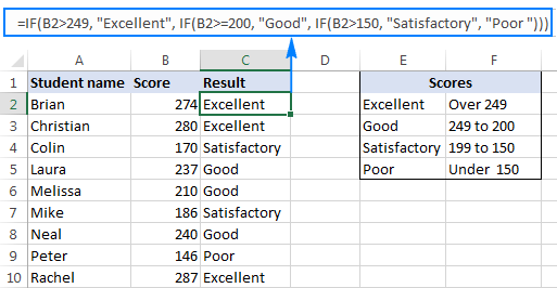
Classic nested IF formula

Understanding Excel nested IF logic

I've heard some people say that Excel multiple If is driving them crazy :) Try looking at it at a different angle:
Nested If formula logic

What the formula actually tells Excel to do is to evaluate the logical_test of the first IF function and, if the condition is met, return the value supplied in the value_if_true argument. If the condition of the 1st If function is not met, then test the 2nd If statement, and so on.

IF(check if B2>=249, if true - return "Excellent", or else
IF(check if B2>=200, if true - return "Good", or else
IF(check if B2>150, if true - return "Satisfactory", if false -
return
"Poor")))

If you need a nested IF formula with wildcard characters (partial match), check out this example: If cell contains, then return different values.

Example 2. Multiple If with arithmetic calculations

Here's another typical task: the unit price varies depending on the specified quantity, and your goal is to write a formula that calculates the total price for any amount of items input in a specific cell. In other words, your formula needs to check multiple conditions and perform different calculations depending on what amount range the specified quantity falls in:

Unit Quantity Price per unit
1 to 10 $20
11 to 19 $18
20 to 49 $16
50 to 100 $13
Over 101 $12

This task can also be accomplished by using multiple IF functions. The logic is the same as in the above example, the only difference is that you multiply the specified quantity by the value returned by nested IFs (i.e. the corresponding price per unit).

Assuming the user enters the quantity in cell B8, the formula is as follows:

=B8*IF(B8>=101, 12, IF(B8>=50, 13, IF(B8>=20, 16, IF( B8>=11, 18, IF(B8>=1, 20, "")))))

And the result will look something similar to this:
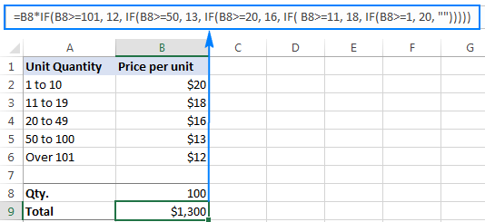
Nested IF formula to perform different calculations on numbers within a certain range

As you understand, this example demonstrates only the general approach, and you can easily customize this nested If function depending on your particular task.

For example, instead of "hard-coding" the prices in the formula, you can reference the cells containing those values (cells B2 to B6). This will enable your users to edit the source data without having to update the formula:

=B8*IF(B8>=101,B6, IF(B8>=50, B5, IF(B8>=20, B4, IF( B8>=11, B3, IF(B8>=1, B2, "")))))
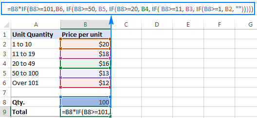
An improved formula with multiple IF functions

Or, you may want to include an additional IF function(s) that fixes an upper, lower or both bounds of the amount range. When the quantity is outside the range, the formula will display an "out of the range" message. For example:

=IF(OR(B8>200,B8<1), "Qty. out of range", B8*IF(B8>=101,12, IF(B8>=50, 13, IF(B8>=20, 16, IF( B8>=11, 18, IF(B8>=1, 20, ""))))))
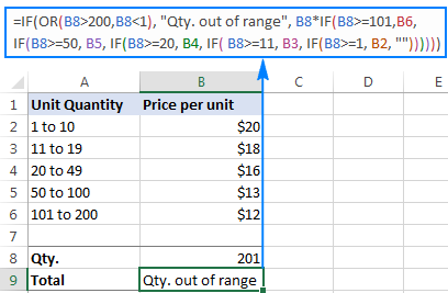
Nested IF's formula with fixed bounds

The nested IF formulas described above work in all versions of Excel. In Excel 365 and Excel 2021, you can also use the IFS function for the same purpose.

Advanced Excel users that are familiar with array formulas, can use this formula that basically does the same thing as the nested IF function discussed above. Though the array formula is far more difficult to comprehend, let along to write, it has one indisputable advantage - you specify the range of cells containing your conditions rather than referencing each condition individually. This makes the formula more flexible, and if your users happen to change any of the existing conditions or add a new one, you will only have to update a single range reference in the formula.

Excel nested IF - tips and tricks

As you have just seen, there is no rocket science in using multiple IF in Excel. The following tips will help you improve your nested IF formulas and prevent common mistakes.

Nested IF limits

In Excel 2007 - Excel 365, you can nest up to 64 IF functions. In older versions of Excel 2003 and lower, up to 7 nested IF functions can be used. However, the fact that you can nest a lot of IFs in one formula doesn't mean you should. Please keep in mind that each additional level makes your formula more difficult to understand and troubleshoot. If your formula has too many nested levels, you may want to optimize it by using one of these alternatives.

The order of nested IF functions matters

The Excel nested IF function evaluates the logical tests in the order they appear in the formula, and as soon as one of the conditions evaluates to TRUE, the subsequent conditions are not tested. In other words, the formula stops after the first TRUE result.

Let's see how it works in practice. With B2 equal to 274, the nested IF formula below evaluates the first logical test (B2>249), and returns "Excellent" because this logical test is TRUE:

=IF(B2>249, "Excellent", IF(B2>=200, "Good", IF(B2>150, "Satisfactory", "Poor")))

Now, let's reverse the order of IF functions:

=IF(B2>150, "Satisfactory", IF(B2>200, "Good", IF(B2>249, "Excellent", "Poor")))

The formula tests the first condition, and because 274 is greater than 150, the result of this logical test is also TRUE. Consequently, the formula returns "Satisfactory" without testing other conditions.

You see, changing the order of IF functions changes the result:
The order of nested IF functions matters

Evaluate the formula logic

To watch the logical flow of your nested IF formula step-by-step, use the Evaluate Formula feature located on the Formula tab, in the Formula Auditing group. The underlined expression is the part currently under evaluation, and clicking the Evaluate button will show you all the steps in the evaluation process.

For example, the evaluation of the first logical test of the nested IF formula shown in the screenshot below will go as follows: B2>249; 274>249; TRUE; Excellent.
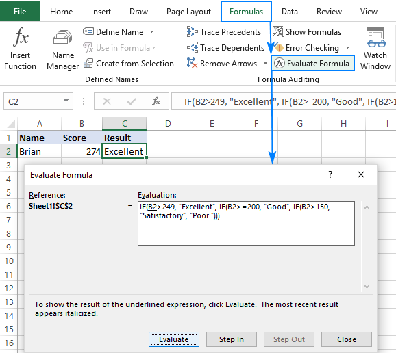
Watch the logical flow of your nested IF formula by using the Evaluate Formula feature.

Balance the parenthesis of nested IF functions

One of the main challenges with nested IFs in Excel is matching parenthesis pairs. If the parentheses do not match, your formula won't work. Luckily, Microsoft Excel provides a couple of features that can help you to balance the parentheses when editing a formula:

  • If you have more than one set of parentheses, the parenthesis pairs are shaded in different colors so that the opening parenthesis matches the closing one.
  • When you close a parenthesis, Excel briefly highlights the matching pair. The same bolding, or "flickering", effect is produced when you move through the formula by using the arrow keys.

Balance the parenthesis of nested IF functions

For more information, please see Match parenthesis pairs in Excel formulas.

Treat text and numbers differently

When building logical tests of your nested IF formulas, remember that text and numbers should be treated differently - always enclose text values in double quotes, but never put quotes around numbers:

Right: =IF(B2>249, "Excellent",…)

Wrong: =IF(B2>"249", "Excellent",…)

The logical test of the second formula will return FALSE even if the value in B2 is greater than 249. Why? Because 249 is a number and "249" is a numeric string, which are two different things.

Add spaces or line breaks to make nested IFs easier to read

When building a formula with multiple nested IF levels, you can make the formula's logic clearer by separating different IF functions with spaces or line breaks. Excel doesn't care about extra spacing in a formula, so you may not worry about mangling it.

To move a certain part of the formula to the next line, just click where you want to insert a line break, and press Alt + Enter. Then, expand the formula bar as much as needed and you will see that your nested IF formula has become much easier to understand.
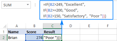
Add line breaks to improve the readability of nested IFs.

Alternatives to nested IF in Excel

To get around the limit of seven nested IF functions in Excel 2003 and older versions and to make your formulas more compact and fast, consider using the following alternatives to nested Excel IF functions.

  1. To test multiple conditions and return different values based on the results of those tests, you can use the CHOOSE function instead of nested IFs.
  2. Build a reference table and a use VLOOKUP with approximate match as shown in this example: VLOOKUP instead of nested IF in Excel.
  3. Use IF with logical functions OR / AND, as demonstrated in the these examples.
  4. Use an array formula like shown in this example.
  5. Combine multiple IF statements by using the CONCATENATE function or the concatenate operator (&). A formula example can be found here.
  6. For experienced Excel users, the best alternative to using multiple nested IF functions might be creating a custom worksheet function using VBA.

This is how you use an If formula in Excel with multiple conditions. I thank you for reading and hope to see you on our blog next week.

Practice workbook for download

Nested If Excel statements (.xlsx file)

635 comments

  1. Hi all, I'm having an issue trying to "stack" multiple possibilities to come up with a text string depending on data in specific cells. Basically, I have Column C1-6, and I'm trying to get a formula where if there is a NAME in cells C1 & C2, the output would be "NAME1 and NAME2"; if there is a NAME in Cells C1, C2 and C3, the output would read "NAME1, NAME2, and NAME3"; if there is a NAME in cells C1-4, the output would be "NAME1, NAME2, NAME3, and NAME4"; et cetera. I can't seem to get past two without messing it up somewhere and would really appreciate some help. Below is the closest I've gotten to making it work but something in there is giving me an incomplete answer after two inputs. Thanks in advance for any advice.

    =Rent!C4&IF(Rent!C7="","",IF(Rent!C10=""," and "&Rent!C7&IF(Rent!C13="","",", "&Rent!C7&", and "&Rent!C10&IF(Rent!C16="","",", "&Rent!C7&", "&Rent!C10&", "&Rent!C13&", and "&Rent!C16&IF(Rent!C19="","",", "&Rent!C7&", "&Rent!C10&", "&Rent!C13&", "&Rent!C16&", and "&Rent!C19)))))

  2. =SUMIF(B21,"=",M21)*OR(B21,"",O21)+B21*B13*3

    How do I take this formula and make it pick one total value?
    Right now it is multiplying all of them together and it either or.

    If the flow is under 556,000 then its =SUMIF(B21,"=",M21)*OR(B21,"",O21)+B21*B13*3

    All together it multiplies them together.
    I need it to pick one that fits.

    can this be achieved in a formula or would I need to do it another way?

    thanks much.

    • Hi,

      I need a formula that help me get data from multiple conditions.

      For Example:

      1.First cell contains (from Data validation) = UNITS & VALUE.

      2.Second cell contains (from Data validation) = TOTAL LEVEL,DEPARTMENT LEVEL,BRAND LEVEL,CLASS LEVEL,ARTICLE LEVEL,PROGRAM LEVEL.

      3.Third cell contains (Lookup from 2nd cell) = If "total" then data must be in total, If "Dept" then Data must be at dept "Dept Level" and carry on..

      I can share sheet as well for reference.

  3. Am having a dataset on google sheet, i want to calculate, employees whose ages are = or less than 20, 30, 40, 45, 50 knowing fully well one column contains the ages of all the employees

  4. Thank you Svetlana ,
    I'm just finishing one of most challenging Complicated formula with 29 Nested IF .

    My advice to Draw a flow chart to build up your logic and your sequence .
    Whatever the Problem is Complected , Once you Build a flowchart , you will figure your way .

  5. I am trying to figure out how to use the IF function to calculate commission, but in a range of sales. There has to be an additional function.

    The difference is the the commission goes down as the sales increase in a range.

    The first $50k pays 4.75%
    The next 51K to $150k pays 3%
    Everything over 150K pays 1.5%

    So, with $1,000,000 of sales
    $50,000.00 @ 4.75% $2,375.00
    $100,000.00 @3% $3,000.00
    $850,000.00 @ 1.5% $12,750.00
    Total Commission $18,125.00

  6. 1st One thousand COD Charge 20 Taka
    Next Per thousand COD charge 8 Taka

    0-1000= 20 Taka
    1001-Above= 8 Taka, Per thousand Charge

    So which formula I used this Case
    Plz hep me

  7. Hello again,
    Further to my recent comment, I have resolved my problem by using the IF, AND functions together.
    Thank you for your posts as I often resolve problems from reading your answers in these pages.
    Many thanks

  8. Hello,
    In columns B and C I have used the IF Function to return the values "High" or "Low".
    Now, from these two columns I need to return the following values in column D.

    B C Value in D
    4 High High Star
    5 High Low Puzzle
    6 Low High Plow horse
    7 Low Low Dog

    I am not sure which function would be best here, thanks in advance.

  9. in if command two value is same and name is different how to solve this problem. for example, if b2=82," Pakistan" ,if b2=82," India" in my sheet both value count is same. how to resolve this issue plz guide.

  10. I don't havve no. but percentages
    18.18%
    18.58%
    15.86%
    15.09%
    19.35%
    16.14%
    I want to use if function fot low, okay, good

  11. I would need your help with the example of product name # XYZ in column A, then column B is Ranking start with 1 and column C with ETA date eg: 3 April 2023 and column D is days of gap and "0" for all with Rank 1. then 2nd line repeated product name # XYZ, Rank - 2 with ETA 5 April 2023, with Gap of 2 days (same product -ETA for Rank 2 minus ETA date of Rank1). How to have the results if product name for column A is same, then compare the gap of the ETA day between rank 1 and 2, if is more than 30 days show the result as high chance and less than 30days with result in low chance. and if days of gap between rank 1 and 2 is same = 0, then move to compare for rank 2 and rank 3.

  12. I have a calculation similar to example 2 above. I cave successfully applied the calculation demonstrated above. However I need to 'layer it', not sure if that is the teccy word!

    I am paid commission, dependent on the total I 'bank' to my employer.
    If I 'bank' up to £4000, I get 55%.
    If I 'bank' up to £8000, I get 55% on the first £4000, then 60% on the second £4k.
    If I 'bank' over £8000 I get 55% on the first £4k, then 60% on the second £4k, then 65% on anything above £8k. How do I create this formula?

    • Hi!
      If I got you right, the formula below will help you with your task:

      =MIN(A1,4000)*55% + MIN(MAX(0,A1-4000),4000)*60% + MAX(0,A1-8000)*65%

  13. I have an Excel sheet that has 1 of 4 possible subjects in cell C3 (English, Maths, History, French) and in cell AD3, I have the "score" which is an average of a number of preceding cells in the same row.

    I am attempting to get a "Pass" or "Fail" result to appear in cell AE3.

    This needs to be based on the following:
    Pass =70%+ for English and Maths
    Pass = 60%+ for French and History

    e.g
    if cell C3 contains "either English or Maths" and the score is more than 70% show "Pass" in cell AE3

    and

    if C3 contains "either French or History" and the score is more than 60% show "Pass" in cell AE3

    Could you please help with a formula to solve this....

      • Thanks for the fast reply.... just tried and this did not work if the C3 cell contained Maths or English and the value in AD3 = >70% any thoughts?

        • Hi!
          The formula I sent to you was created based on the description you provided in your first request. I can't check this formula because I don't have your data. I gave you a link to an article with which you can solve the problem.

          • Thanks, I can see the issue, my number data in AD3 was not formatted as %, after removing the % from the formula, this now works.

            As the data in C3 could contain any of the 4 subjects, would it be possible to have formula check for the subject and apply the checking for pass score?

    • If d2=1 and e2>99, "fail", "pass", if d2>1 and e2 is >249 "fail", "pass".

      • Sorry, can you help me create a formula with these conditions?

        If d2=1 and e2>99, "fail", "pass", if d2>1 and e2 is >249 "fail", "pass".

  14. Hi,
    I am trying to write a formula that states:
    IF cell C1 = Daily then do this sum ((D1/60)*7.5))
    IF cell C1 = Weekly then do this sum ((D1/60)*37.5))
    IF cell C1 = Fortnightly then do this sum ((D1/60)*75))
    IF cell C1 = Monthly then do this sum ((D1/60)*162.5))
    IF cell C1 = Quarterly then do this sum ((D1/60)*487.5))
    IF cell C1 = Yearly then do this sum ((D1/60)*1950))

    Can anyone help please?

    Thanks
    Suzy

      • Thank you for coming back so quick.
        I have tried to simply a little and have put the below function in but it keeps coming back with the error #NAME? in the cell:
        =IFS(D9="Daily",(AF9/7.5),D9="Weekly",(AF9/37.5),D9="Fortnightly",(AF9/75),D9="Monthly",(AF9/162.5),D9="Quarterly",(AF9/487.5),D9="Yearly",(AF9/1950))

        • I also only have excel 2016 so i am not sure it recognises IFS

        • Hi!
          IFS function is available only in Excel 365, Excel 2021 and Excel 2019. If this fuction is not available for you, use the recommendations from the article above. You only have 6 nested IFs.

          =IF(D9="Daily",AF9/7.5,IF(D9="Weekly",AF9/37.5,IF(D9="Fortnightly",AF9/75,IF(D9="Monthly",AF9/162.5,IF(D9="Quarterly",AF9/487.5,IF(D9="Yearly",AF9/1950,""))))))

  15. Thank you for this concise answer!

    Slava Ukraini!

  16. Thank you for this information. Unfortunately, I was not able to get my formula to work.

    I am trying to get the following to happen. For column Y, the value is one of the following statuses: NEW, QUEUED, INPROG, REJECTED, CLOSED or (blank), For the statuses of NEW, QUEUED, INPROG I need the value returned to say "SR NEED COMPLETED". for status of REJECTED, I need the value returned to say "SR NOT NEEDED". for the status of CLOSED or (if it is blank), I need the value returned to say "SR NEEDED"

    My formula is =IF(OR(Y10="NEW", Y10="QUEUED",Y10="INPROG"), "SR NEED COMPLETED",(IF(Y10="REJECTED"),"SR NOT NEEDED","SR NEEDED"))))

    I've also tried this formula
    =(IF(OR(Y10="NEW",Y10="QUEUED",Y10=”INPROG”),"SR NEED COMPLETED",(IF(Y10="REJECTED”),"SR NOT NEEDED”,(IF(OR(Y10="CLOSED",Y10="")"SR NEEDED"))))))

    Any help would be appreciated.

    • Hi!
      If I understand your task correctly, try the following formula:

      =IF(OR(Y10="NEW",Y10="QUEUED",Y10="INPROG"),"SR NEED COMPLETED",IF(Y10="REJECTED","SR NOT NEEDED","SR NEEDED"))

      • This worked perfectly for me. Thank you.

  17. I have a column which contains numbers separated by a ";" delimiter. Each row has a different number of values. I wish to substitute these numbers (depending upon where they lie within a range) by text and trying to get them in an adjacent cell.

    What I am doing right now is converting text to columns and then applying the formula IFS(AND(A6>=-200,A6=201,A6<=1500),"TS1500",AND(A6=-1500),"TS1500") to each cell. Thus, if I have 50 delimited items in one cell, it results in 50 columns, and then 50 more columns to apply the formula, one per cell. Is there any other way to get this done?

    Current situation:
    What I have is col A. Then split into cols B-F. Then formulas are put in cols G-K, which are combined in col L.

    A B C D E F G H I J K L
    168; -765; 1400; -18; 2400 168 -765 1400 -18 2400 TS200 TS1500 TS1500 TS200 #N/A TS200;TS1500;TS1500;TS200;#N/A
    -98; 63 -98 63 TS200 TS1500 TS200;TS1500

    Preferred result:
    What I would like is a column B containing all the values separated by “;”

    A B
    168; -765; 1400; -18; 2400 TS200;TS1500;TS1500;TS200;#N/A
    -98; 63 TS200;TS1500

    • Hi!
      I'm really sorry, we cannot help you with this. You can replace values for multiple conditions using a formula for each cell.

      • Thank you

  18. Hi I'm hoping someone one on this forum can help me,
    I have an excel spreadsheet which I want to tell me which stage I am in. For instance if text or date is entered in B2 write "Stage 1" in cell A2, if a text or date is entered in cell C2 change to "Stage 2" etc. Here is a copy of the code I have used that isn't working

    =IF(AND(ISTEXT(B2)),"Stage 1"), IF(AND(ISTEXT(C2)),"Stage 2"), IF(AND(ISTEXT(D2)),"Stage 3"),IF(AND(ISTEXT(E2)),"Stage 4"), IF(AND(ISTEXT(F2)),"Stage 5")

    Any help would be appreciated :)

    • Hi!
      Please try the following formula:

      =IF(ISTEXT(B2),"Stage 1",IF(ISTEXT(C2),"Stage 2",IF(ISTEXT(D2),"Stage 3",IF(ISTEXT(E2),"Stage 4",IF(ISTEXT(F2),"Stage 5")))))

  19. Hi!
    I'm trying to check for criteria met for partner Status. If a company has status as "Bronze" they need to have 1 person or more that have passed a Test, if they have Status "Plata" at least 2 people must have passed a test and if their status is "Oro" 3 people minimum must have passed a test.
    Column E should say yes or not if the criteria is met. I have that Column C gives the partner Status as Text and Column D has the number of people that have passed the test.
    I have the formula when I have only one level:
    Level Passed Met Criteria
    Bronze No
    Bronze 1 Yes
    Bronze 4 Yes
    Using this
    =IF(AND(C67="Bronze", D67>=1), "Yes", "No")
    I want to be able to check if another level (Levels Plata and Oro are in text form in Column C as well) is assigned the test criteria is met
    here is what I've Tried:
    =If((AND(C26="Bronze", D26>=1), "Yes", "No"),if(and(C26="Plata", D26>=2), "Yes", "No",if(and(C26="Oro",D26>=3), "Yes","No")))

    I've also tried with OR

    Thank you in advance for your help!

    • Hello!
      If I understand your task correctly, try the following formula:

      =IF(AND(C26="Bronze", D26>=1), "Yes",IF(AND(C26="Plata", D26>=2), "Yes",IF(AND(C26="Oro",D26>=3), "Yes","No")))

  20. I have a nested If function formula with vlookups that is returning a false value.
    In short, I have multiple bank accounts, where is the final 4 numbers is the bank account = a set number, I need the vlookup to draw information from another worksheet.

    =IF(X3="","",IF(X3="2121",IFERROR(VLOOKUP(N3,'Monthly CR Data'!T:AA,8,FALSE),IF(X3=2089,VLOOKUP(N3,'Monthly CR Data'!U:AA,7,FALSE),"Not Reconciled"))))

    Problem is, it works for the '2121' account, but the '2089' account pulls back a false value, rather than doing the VLOOKUP in the cells specified.

    Any help would be greatly appreciated

    • Hi!
      I can't check the formula that contains unique references to your workbook worksheets. Try adding quotes in the second IF condition. X3="2089"

  21. hi! i have am trying to capture multiplying by the higher value.
    i have, minimum order Quantity (MOQ) in A2, and i have the customers required amount in B2.

    and i have unit price in C2

    so when MOQ is higher, multiply MOQ x unit price, but when customer requirement is higher, multiply requirement by unit price.

  22. in this formula we able to merge 2 column value how can we merge multiple value of column B formula is =IF(A3A2,B3,B3 &","&B2)

    Thanks for your support in advance.

    • Hi!
      Add the values you want to merge to the formula. For example

      =IF(A3>A2,B3,B3 &","&B2&","&B4)

      If this is not what you wanted, please describe the problem in more detail.

  23. Good day!

    Status cell to be changed by checking 5 different cells:

    My status is in cell B11 and the cells to check values are C11, D11, E11, F11, G11.

    if any one of the cells have "No" or "Active" then the status should be "In-Progress". if all the cells have "N/A" then status should be "N/A". if all the cells have "Yes" then status should be "Complete".

    How to check multiple cells in one time and update the status? Kindly help. Thanks for the help!

    Used below formula but feels like too long!
    =IF(C11="NO","IN-PROGRESS",IF(C11="Active","IN-PROGRESS",IF(D11="NO","IN-PROGRESS",IF(D11="Active","IN-PROGRESS",IF(E11="NO","IN-PROGRESS",IF(E11="Active","IN-PROGRESS",IF(F11="NO","IN-PROGRESS",IF(F11="Active","IN-PROGRESS",IF(G11="NO","IN-PROGRESS",IF(G11="Active","IN-PROGRESS",IF(H11="NO","IN-PROGRESS",IF(H11="Active","IN-PROGRESS",IF(I11="NO","IN-PROGRESS",IF(I11="Active","IN-PROGRESS",IF(J11="Active","IN-PROGRESS",IF(J11="NO","IN-PROGRESS","COMPLETE"))))))))))))))))

  24. Good day!

    Status cell to be changed by checking 5 different cells:

    My status is in cell B11 and the cells to check values are C11, D11, E11, F11, G11.

    if any one of the cells have "No" then the status should be "In-Progress". if all the cells have "N/A" then status should be "N/A". if all the cells have "Yes" then status should be "Complete".

    How to check multiple cells in one time and update the status? Kindly help. Thanks for the help!

    • Hi!
      To check all values, use the SUM function

      =IF(SUM(--(C11:G11="No")),"No",IF(SUM(--(C11:G11="Yes"))=5,"Complete",IF(SUM(--(C11:G11="N/A"))=5,"N/A","")))

      Also follow the instructions from the article above.

  25. Could you maybe help me with a formula for this problem?

    I have a spreadsheet with a lot of data, and I will like for you to help me with he below

    I have over 6K members that were prescribed medications during years 2021 and 2022.

    I want to know which members had medicine prescribed during 2021 only, 2022 only or both (2021 & 2022). I want to have a formula that displays "2021", "2022" or "BOTH"

    I have the below columns among all the data:

    Prescribed date (using format YYY-MM-DD)
    Prescribed Year (YYYY)
    Person Id (Unique ID numbers) - This column has all ID numbers for members that received medications, meaning that is possible one member ID could be in this column multiple times if this person got medications more than once. Example below

    ID Fill Date Year What I'm looking for
    12345 2022-05-05 2022 BOTH
    12345 2021-01-03 2021 BOTH
    01123 2022-03-09 2022 2022
    05486 2021-01-25 2021 2021
    23546 2021-05-30 2021 2021
    01123 2022-04-09 2022 2022

    • [ ID ] [Fill Date] [Year] [What I'm looking for]
      12345 2022-05-05 2022 BOTH
      12345 2021-01-03 2021 BOTH
      01123 2022-03-09 2022 2022
      05486 2021-01-25 2021 2021
      23546 2021-05-30 2021 2021
      01123 2022-04-09 2022 2022

  26. =IFS(I7="AC","CEEW4",I7="WM","CEEW3",I7="REF","CEEW2",I7="","")
    this similar formula I need in Excel

  27. I can figure out why the formula is breaking. The data columns it's pulling from are all validation lists.

    =UPPER("1 x 1 "&[@[Year & Quarter]]&" "&C6&" "&IF([@Site]="Facebook","FB",IF([@Site]="twitter","TW",IF([@Site]="TikTok", "TikTok",IF([@Site]="Reddit","Reddit", IF([@Site]="snapchat","Snapchat",IF([@Site]="Pinterest","Pinterest","No Social Platform"))))))&" "&[@[Audience Type Category
    (Automated when Salesforce Audience ID is present)])"&[@[Analytics Report Placement Name
    (Freehand/Use "NA" if blank)]&" "&[@[Opt Descriptor
    (Freehand/Use "NA" if blank)])

  28. Hi Alexander,

    could you maybe help me with a formula for this problem?
    I want to check how many deliveries were made on time for 3 separate categories. There are deliveries that are emergency , priority and regular.
    Emergency deliveries should be delivered within a day so x<=1
    Priority deliveries should be delivered within 2 days so y<=2
    Regular deliveries should be delivered within 7 days so y<=7
    If it took more then the days mentioned above, delivery is considered late.

    My data set looks like the following:
    x - 1
    y - 5
    z - 6
    z - 0
    z - 2
    y - 0
    x - 1
    x - 0
    x - 0

    How can I combine this question into one formula?

      • Hi Alexander, I think it is not exactly what I am looking for.
        I managed to make this formula for 1 category (emergency deliveries) =IF(AND(A2="Emergency",B2<=1),"1","0"). In this way I am asking excel to show me emergency deliveries that are delivered either on time (1) or too late (0) which in this case it is on time if it is delivered within a day. How can I add the other two categories? Priority and regular. Priority should be delivered within 2 days and Regular within 7 days. I thought I need to and two more if functions but if I do so I get #value

          • Assume this is the data set:
            Emergency -3 days
            Priority - 7 days
            Regular - 8 days
            Priority - 9 days
            Emergency - 0 days
            Regular - 1 day
            Regular - 10 days
            Emergency - 1 day

            Emergency deliveries should be delivered within a day so Emergency <=1
            Priority deliveries should be delivered within 2 days so Priority <=2
            Regular deliveries should be delivered within 7 days so Regular <=7

            I want excel to tell me which orders were delivered on time and which too late based on their urgency and the above mentioned conditions. I was able to make this formula: =IF(AND(A2="Emergency",B2<=1),"1","0") but I don't know how to add the other delivery types.
            Your help is much appreciated

              • Alexander,

                Thank you so much for your help. it is indeed what I needed!

  29. HI,

    i wan to solve below table

    Site id status Final status
    BHAIYATHAN 5|1 UP Up If first and last up then final status all column up
    BHAIYATHAN 5|2 Down Up
    BHAIYATHAN 5|3 Down Up
    BHAIYATHAN 5|4 Down Up
    BHAIYATHAN 5|5 Down Up
    BHAIYATHAN 5|6 Down Up
    BHAIYATHAN 5|7 Down Up
    BHAIYATHAN 5|8 Down Up
    BHAIYATHAN 5|9 Down Up
    BHAIYATHAN 5|10 UP Up

    Site id status Final status
    BHAIYATHAN 5|1 Down Down If status Down Then Final Status is actul of status
    BHAIYATHAN 5|2 Down Down
    BHAIYATHAN 5|3 Down Down
    BHAIYATHAN 5|4 Down Down
    BHAIYATHAN 5|5 Down Down
    BHAIYATHAN 5|6 Down Down
    BHAIYATHAN 5|7 Down Down
    BHAIYATHAN 5|8 Down Down
    BHAIYATHAN 5|9 Down Down
    BHAIYATHAN 5|10 UP Up

    Site id status Final status
    BHAIYATHAN 5|1 Up UP
    BHAIYATHAN 5|2 Down Down
    BHAIYATHAN 5|3 Down Down
    BHAIYATHAN 5|4 Down Down
    BHAIYATHAN 5|5 UP UP
    BHAIYATHAN 5|6 Down Down
    BHAIYATHAN 5|7 Down Down
    BHAIYATHAN 5|8 Down Down
    BHAIYATHAN 5|9 Down Down
    BHAIYATHAN 5|10 Down Down If last down Then All final status Actual of status

  30. Hi
    I want to write an IF that can be used for several ranges of Excel, for example:
    scores result criteria
    78 scores result
    34 <30 Fail
    49 30-50 III Div
    10 50-70 II Div
    89 70-90 I Div
    28 90+ Incredible
    80
    77
    64
    98
    thanks pirooz

  31. Hi Alexander,

    Please help me with my following problem.
    Cell A2 = 300
    B2 = 100
    C2 = 500

    =IF(A2>B2, A2,B2, IF A2>C2, A2,C2, IF C2>B2, C2,B2)))

    The true result will only show the first and the second IF.

    Thank you in advance.

    • Hi!
      Based on your description, it is hard to completely understand your task. I don't know what result you want to get. However, I’ll try to guess and offer you the following formula:

      =IF(A2>B2,A2,IF(A2>C2,A2,IF(C2>B2,C2,B2)))

      Please re-check the article above since it covers your task.

      • Hi Alexander,

        Thank you for the reply. Sorry if I didn't explain the problem well, but you got I what I mean. :)

        I tried your formula, however, it only shows that C2 is greater than A2 if B2 is greater than A2. But if B2 is lower that A2, then the answer in the formula is A2 is greater than C2 & B2 which should be C2 is greater than A2 of B2.

        Sorry again to bother you but hopefully you can help me with this coz I'm not really good in excel.

        Thank you so much!

        • Hi!
          I just corrected the syntax errors in your formula. But I still don't understand what result you want to get. All detailed instructions are in the article above. Or describe in detail the desired result.

  32. Hello I have been stuck on this IF statement for three days now and I keep getting invalid or the pound sign, as well as just the equation I'm inputting to still be there with nothing being done. This one is kind of weird to do, for me: I have to make a nest statement for when I can go to the beach the set up is below. I can only go on Friday, the weather has to be nice and I have to have at least $500. That's the only numeric number but I set it up different ways so many times that I've lost sight of what and how to use the and, can't... =IF(A4<=Friday?, "Yes", IF(A4=,Bad Weather, "No", IF(A4<=$500, "Can't Go"))) A4 is the first cell with Friday in it. Can you tell me what I'm doing wrong? I've watched a couple of youtube vids, and articles but the formulas I try yield the same result: Nothing. Please and thank you for your time.

    Friday with an drop down arrow
    Friday
    Anyday

    Sunny and warm
    Sunny and warm
    Nasty

    $500

  33. Hello

    I cannot figure out how to fix this IF AND NESTED formula. Please help.

    =IF(AND(R2>=19.01, R2=21.01, R2<=23, 70, IF(R2<=23.01, 75, " " )))

  34. Hi,
    Can you help me with this calculation?
    I want to calculate the commission (3%,5%,7% etc) based on the total sales in location i16

    =IF(i162000=4000,"i16"/100*5,IF(i16>4000=6000,"i16"/100*7)))

    Thanks in advance

  35. Hi so this is my current formula

    =IF(OR([@[FULL NAME]]="Player 1",[@[FULL NAME]]="Player 2",[@[FULL NAME]]="Player 3",[@[FULL NAME]]="Player 4",[@[FULL NAME]]="Player 5",[@[FULL NAME]]="Player 6", [@[FULL NAME]]="Player 7", [@[FULL NAME]]="Player 8"),"DEF")

    I'm wanting to add two other IF OR onto the formula, so if player 9, player 10, player 11 then itll be MID and then for players 12, 13, 14 itll be 'ATT'.

    Does anyone know how I could add these on?

    Thanks in advance!

  36. Good morning - I am looking for a simplified formula to calculate all of the possible outcomes between 4 categories (East, Midwest, South, and West) and their 3 potential ratings (Low, Medium, High). The current formula - which has accounted for all possible outcomes - has produced 81 levels of nesting (3 x 3 x 3 x 3 = 81), which obviously is too large and cannot be entered. I was wondering if using IFS instead of nested IFs might work? Any suggestions would be tremendously appreciated - thanks!

  37. Hi,

    What can be the formula for this?
    Since I have 140k line items, how can I group the Order No. based on the Items?
    Let's say classification is not available and I want to group the order no. with multiple types of goods as "Mixed Items".

    Order No. Item Classification
    1 Fish Mixed Items
    1 Veggies Mixed Items
    1 Fruits Mixed Items
    1 Rice Mixed Items
    2 Fish Seafoods Only
    2 Fish Seafoods Only
    2 Fish Seafoods Only
    3 Bread Breads Only
    3 Bread Breads Only

    Thanks in advance!

    • Hello!
      If I understand your task correctly, try the following formula:

      =IF(COUNTA(UNIQUE(FILTER($B$1:$B$100,$A$1:$A$100=A1)))=1,"Mixed items","")

      or

      =IF(IFERROR(ROWS(UNIQUE(FILTER(B1:B100,$A$1:$A$100=A1))), 0)=1,"Mixed items","")

      For more information, please visit: Count unique values with criteria.

  38. I have a column of cells with drop-down options of "Complete", "In Progress", "Not Started", and "Backlog." J6 - J25 specifically.
    I have a cell that I am attempting to display the overall progress as a percentage (located at H3).
    How do I get a selection of "Complete" to contribute to the percentage as a 100% value, the "In Progress" to contribute to the percentage as a 50% value and all others 0.
    For example: J6-8 says, "Complete" "Complete" "Complete"... then H3 will say "100%"
    or "Complete", "Not Started" will have H3 showing "50%"

    • Hi!
      Your description of the problem and the example do not match, but the formula could be something like this -

      =IF(SUM(--(J6:J8="Complete"))=3,100%,IF(SUM(--(J6:J8="In progress"))=3,50%,""))

      About using double dash (--) with boolean values learn more in example 3 in the article - SUMPRODUCT and SUMIFS in Excel. I hope my advice will help you solve your task.

  39. Hi

    =IF($G60,$G$4,)&" "&IF($H60,$H$4,)&" "&IF($I60,$I$4,)

    G6, H6, I6 = Sales
    G4, H4, I4 = Place

    Is there any other formula which I can use in place of above formula.

    Thanks

  40. Hi Alex
    I have one column (E) where i have the percentage calculated.
    Then i have a Target Points Colums (B) with numbers 1-5
    now i need to set a condition in COlumn F, where if the average is 100% and above i need to add 1 to the value in column B

    100%-110% plus 1 90%-100% minus 1
    110%-120% plus 2 80%-90% minus 2
    120%-130% plus 3 70%-80% minus 3
    130%-140% plus 4 60%-70% minus 4
    140%-150% plus 5 50%-60& minus 5

    Thanks
    A

      • Hello, please help with any formula suggestions for what I'm trying to do -
        For each dollar of new income (as shown in cell D13) between $140 and $220, calculate an abatement of .20cents per dollar, and deduct this from current income (found in D7)....
        Then for each dollar of new income (D13) above $220, calculate an abatement of .50cents per dollar, and also deduct this from current income (found in D7).
        My version of excel is older; can't use SUMIFS.
        (sorry to hijack this thread, can't find where to start a new comment)

  41. Would like some advice about a nested IF formula. The formula I have written is: =IF(L2>0,L2,IF(K2>0,K2,IF(J2>0,J2,IF(I2>0,I2,G2))))
    with the intention that the latest filled column from I to L should be copied over to a new column and if there's nothing in I-L then column G should be copied instead. The formula works if column L is filled in and SOMETIMES if there's only column G to copy but not for any other scenarios.
    Example:
    G= 7
    I = 9
    J= 11
    K = Blank
    L = Blank
    M with formula should show 11

    I can't work out what I've done wrong!

    • Hello!
      Use the INDEX+MATCH functions to find the last non-empty cell in a range. The following tutorial should help: How to use INDEX and MATCH in Excel.
      Please try the following formula -

      =INDEX(I1:L1,,MATCH(1E+20,I1:L1,1))

      =IFERROR(INDEX(I1:L1,,MATCH(1E+20,I1:L1,1)),G1)

      I hope I answered your question.

      • Yes!!! It worked. Thank you. :)

  42. Hi,

    I want to sort company revenue with the following conditions:

    $250M

    How do I turn this into a nested IF formula? Or do I use another type of formula?

  43. Please support me for following XL formula-
    IF 10000, he is ultra-poor
    IF 10001 to 15000, he is poor
    IF 15001 to 25000, he is middle class

    Thank you

  44. I am trying to do a nested if, and it is telling me I have too many arguments. In cell w2, i am inputting the word "yes", "no", or "probation". I wrote this formula. I am not sure where I have an error, Please help.

    =if(w2, "yes", "APR Complete",
    IF(w2, "no", "APR Needed",
    IF(w2, "probation", "Not Applicable")))

  45. Hi
    Thanks for an excellent article.
    I have successfully managed to get the correct results for the first 3 conditions below. However with regards to IF(AD2>-10,"Big Loss", if the number is greater than -10, it still returns loss instead of "Big Loss"
    What can I do to correct this in the formula below.
    =IF(AD2>=10,"Big Profit",IF(AD2>0,"Profit",IF(AD2<=0,"Loss",IF(AD2<=-10,"Big Loss"))))
    Many thanks,
    Radley

  46. Hi,

    How to get the formula for the following scenarios

    Qty Value Rate Rate 2 Required
    18,508 25,96,571 140 - 140
    21,716 14,15,208 65 225 65

  47. One number is inputted into column A in either A1, A2 or A3 and then that number is also displayed in column B in either B 1, B2 or B3. But which cell it shows in column B should depend on both the value of the number and the cell in column A it was entered into.

    If A1 is lower than 0 then the number is displayed in B3.
    If A1 is 0-100 then the number is displayed in B1.
    If A1 is over 100 then the number is displayed in B2.

    If A2 is lower than 0 then the number is displayed in B1.
    If A2 is 0-100 then the number is displayed in B2.
    If A2 is over 100 then the number is displayed in B3.

    If A3 is lower than 0 then the number is displayed in B2.
    If A3 is 0-100 then the number is displayed in B3.
    If A3 is over 100 then the number is displayed in B1.

    Any idea on how to program this in excel?

  48. Hi I need to calculate the following

    If car is 1200cc or lower the and the following will apply and if the car is 1200 of higher the following will apply. Any help would be appreciated

    1200cc or lower

    up to 1500KM .3795 per KM
    1501 to 14000KM .4109 per km
    14001 to 25000 .2550 per km

    1201cc or higher
    up to 1500KM .3986per KM
    1501 to 14000KM .4109 per km
    14001 to 25000 .2550 per km

    Your help would be greatly appreciated on this

    Ollie

  49. Question. I have been racking my brain all night on this.

    I have 3 pieces of information that are linked to a master table on another sheet.

    I have A1 - Date Assigned
    I have A2 - Goal date
    I have A3 - Date completed

    I want to be able to put in a date into assigned and on my tracker have it read "A" on my master tracker
    I am able to calculate a goal date, but want it to show "D" if is goes past the goal date referenced in A2 on the master tracker.
    And then I want to be able to put a date in A3 and then have it read "X" for when there is a date listed for completion on my master tracker.

    In addition, I want to be able to notice if there are no dates in either A1, A2, or A3 that it just shows blank on the master tracker.

    I hope that is enough information to go off of.

    Thanks for your help.

    • Also worth noting I have tried to get a formula using =IF(Z6>=TODAY()-(W6*7),AJ6,IF(Z6<=TODAY()-(W6*7),AJ7,IF(AE6,AJ8, "")))

      But it will only do the first two it won't allow my third argument to go.

  50. I have a calculation between 2 cells where, based on the sum, the value should change. If not true, then the value should = the calculated sum. This is the latest attempt but not working. Thanks in advance !

    if(H39*0.5)+(H41*0.5)=1.0,"1", if(h39*.05)+(h41*0.5)=2.0,"2", if (h39*.05)+(h41*0.5)=3.0,"3")))

    • Hi!
      I fixed the errors in the syntax of the IF function

      =IF((H39*0.5)+(H41*0.5)=1,1, IF((H39*0.05)+(H41*0.5)=2,2, IF((H39*0.05)+(H41*0.5)=3,3)))

      • Hello, and thank you so much! Getting closer but not quite there.

        The problem I have is the results field is formatted with a decimal. When the result is a whole number I do not want the .0 . I have solved for this by using "". However, if the result is not a whole number (1,2, 3.) then I need the calculation to show the results "as is" ( e.g. 0.5). Here is my latest attempt but still not working. Wondering if is should use "or"?... Thanks again!

        =IF(H39*0.5+H41*0.5=1,"1",H39*0.5+H41*0.5),IF(H39*0.5+H41*0.5=2,"2",H39*0.5+H41*0.5),IF(H39*0.5+H41*0.5=3,"3",H39*0.5+H41*0.5)

          • Hello again and thank you so much for your quick reponse!

            Wonderful! I'm going to go with the cell format change to "General". I learned more about the nested IF statement through this exchange but it simplifies the formula, so thank you!

            Have a wonderful day!

Post a comment


Thank you for your comment!
When posting a question, please be very clear and concise. This will help us provide a quick and relevant solution to
your query. We cannot guarantee that we will answer every question, but we'll do our best :)