The tutorial explains how to multiply in Excel by using the multiplication symbol and functions, how to create a formula for multiplying cells, ranges or entire columns, how to multiply and sum, and more.
While there is no universal multiplication formula in Excel, there exist a few different ways to multiply numbers and cells. The below examples will teach you how to write a formula best suited for your specific task.
Multiply in Excel by using multiplication operator
The easiest way to do multiplication in Excel is by using the multiply symbol (*). With this approach, you can quickly multiply numbers, cells, entire columns and rows.
How to multiply numbers in Excel
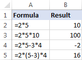
To make the simplest multiplication formula in Excel, type the equals sign (=) in a cell, then type the first number you want to multiply, followed by an asterisk, followed by the second number, and hit the Enter key to calculate the formula.
For example, to multiply 2 by 5, you type this expression in a cell (with no spaces): =2*5
As shown in the screenshot below, Excel allow performing different arithmetic operations within one formula. Just remember about the order of calculations (PEMDAS): parentheses, exponentiation, multiplication or division whichever comes first, addition or subtraction whichever comes first.
How to multiply cells in Excel
To multiply two cells in Excel, use a multiplication formula like in the above example, but supply cell references instead of numbers. For example, to multiply the value in cell A2 by the value in B2, type this expression:
=A2*B2
To multiply multiple cells, include more cell references in the formula, separated by the multiplication sign. For example:
=A2*B2*C2

How to multiply columns in Excel
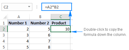
To multiply two columns in Excel, write the multiplication formula for the topmost cell, for example:
=A2*B2
After you've put the formula in the first cell (C2 in this example), double-click the small green square in the lower-right corner of the cell to copy the formula down the column, up to the last cell with data:
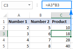
Due to the use of relative cell references (without the $ sign), our Excel multiply formula will adjust properly for each row:
In my opinion, this is the best but not the only way to multiply one column by another. You can learn other approaches in this tutorial: How to multiply columns in Excel.
How to multiply rows in Excel
Multiplying rows in Excel is a less common task, but there is a simple solution for it too. To multiply two rows in Excel, just do the following:
- Insert a multiplication formula in the first (leftmost) cell.
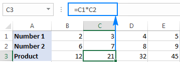
In this example, we multiply values in row 1 by the values in row 2, beginning with column B, so our formula goes as follows:
=B1*B2 - Select the formula cell, and hover the mouse cursor over a small square at the lower right-hand corner until it changes to a thick black cross.
- Drag that black cross rightward over the cells where you want to copy the formula.

As with multiplying columns, the relative cell references in the formula change based on a relative position of rows and columns, multiplying a value in row 1 by a value in row 2 in each column:
Multiply function in Excel (PRODUCT)
If you need to multiply multiple cells or ranges, the fastest method would be using the PRODUCT function:
Where number1, number2, etc. are numbers, cells or ranges that you want to multiply.
For example, to multiply values in cells A2, B2 and C2, use this formula:
=PRODUCT(A2:C2)
To multiply the numbers in cells A2 through C2, and then multiply the result by 3, use this one:
=PRODUCT(A2:C2,3)
The screenshot below shows these multiplication formulas in Excel:

How to multiply by percentage in Excel
To multiply percentages in Excel, do a multiplication formula in this way: type the equals sign, followed by the number or cell, followed by the multiply sign (*), followed by percentage.
In other words, make a formula similar to these:
- To multiply a number by percentage:
=50*10% - To multiply a cell by percentage:
=A1*10%
Instead of percentages, you can multiply by a corresponding decimal number. For example, knowing that 10 percent is 10 parts of a hundred (0.1), use the following expression to multiply 50 by 10%: =50*0.1
As shown in the screenshot below, all three expressions yield the same result:

How to multiply a column by a number in Excel
To multiply a column of numbers by the same number, proceed with these steps:
- Enter the number to multiply by in some cell, say in A2.
- Write a multiplication formula for the topmost cell in the column.
Assuming the numbers to be multiplied are in column C, beginning in row 2, you put the following formula in D2:
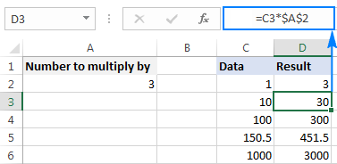
=C2*$A$2It is important that you lock the column and row coordinates of the cell with the number to multiply by to prevent the reference from changing when you copy the formula to other cells. For this, type the $ symbol before the column letter and row number to make an absolute reference ($A$2). Or, click on the reference and press the F4 key to change it to absolute.
- Double-click the fill handle in the formula cell (D2) to copy the formula down the column. Done!
As you can see in the screenshot below, C2 (relative reference) changes to C3 when the formula is copied to row 3, while $A$2 (absolute reference) remains unchanged:
If the design of your worksheet does not allow an additional cell to accommodate the number, you can supply it directly in the formula, e.g.: =C2*3
You can also use the Paste Special > Multiply feature to multiply a column by a constant number and get the results as values rather than formulas. Please check out this example for the detailed instructions.
How to multiply and sum in Excel
In situations when you need to multiply two columns or rows of numbers, and then add up the results of individual calculations, use the SUMPRODUCT function to multiply cells and sum products.
Supposing you have prices in column B, quantity in column C, and you want to calculate the total value of sales. In your math class, you'd multiply each Price/Qty. pair individually and add up the sub-totals.
In Microsoft Excel, all these calculations can be done with a single formula:
=SUMPRODUCT(B2:B5,C2:C5)
If you wish, you can check the result with this calculation:
=(B2*C2)+(B3*C3)+(B4*C4)+(B5*C5)
And make sure the SUMPRODUCT formula multiplies and sums perfectly:

Multiplication in array formulas
In case you want to multiply two columns of numbers, and then perform further calculations with the results, do multiplication within an array formula.
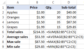
In the above data set, another way to calculate the total value of sales is this:
=SUM(B2:B5*C2:C5)
This Excel Sum Multiply formula is equivalent to SUMPRODUCT and returns exactly the same result (please see the screenshot below).
Taking the example further, let's find an average of sales. For this, just use the AVERAGE function instead of SUM:
=AVERAGE(B2:B5*C2:C5)
To find the largest and smallest sale, use the MAX and MIN functions, respectively:
=MAX(B2:B5*C2:C5)
=MIN(B2:B5*C2:C5)
To complete an array formula properly, be sure to press the Ctrl + Shift + Enter combination instead of Enter stroke. As soon as you do this, Excel will enclose the formula in {curly braces}, indicating it's an array formula.
The results might look something similar to this:
That's how you multiply in Excel, it doesn't take a rocket scientist to figure it out :) To have a closer look at the formulas discussed in this tutorial, feel free to download our sample Excel Multiplication workbook.
How to quickly do any calculations in Excel
If you are a novice to Excel and are not comfortable with multiplication formulas yet, our Ultimate Suite will make things a lot easier for you. Among 70+ cute features, it provides the Calculation tool that can perform all basic mathematic operations, including multiplication, in a mouse click. Let me show you how.
Supposing you have a list of net prices and you want to know the corresponding VAT amount. No big deal if you know how to calculate percentages in Excel. If you don't, have the Ultimate Suite do the job for you:
- Copy the prices to the VAT column. You need to do this because you don't want to override the original values in the Price column.
- Select the copied prices (C2:C5 in the screenshot below).
- Go to the Ablebits tools tab > Calculate group, and do the following:
- Select the percentage symbol (%) in the Operation box.
- Type the desired number in the Value box.
- Click the Calculate button.

That's all there is to it! You will have the percentages calculated in a heartbeat:

In a similar manner, you can multiply and divide, add and subtract, calculate percentages, and more. All you have to do is select an appropriate operator, for example the multiply symbol (*):

To perform one of the recent calculations to another range or column, just click the Apply Recent button, and pick the operation:

The results of all calculations done with the Ultimate Suite are values, not formulas. So, you are free to move or copy them to another sheet or workbook without worrying about updating formula references. The calculated values will remain intact even if move or delete the original numbers.
If you are curious to learn more about this and many other time-saving tools included with the Ultimate Suite for Excel, you are welcome to download 15-day trial version.
I thank you for reading and hope to see you on our blog next week!
 by
by
134 comments
multiplication function for these cells: N11, N12, N13, E14, and E15
Thank you!
My problem is simple, in A column is a, b, c, d, e, f, g repeate randomly up to millions, corresponding value 3, 5, 4, 6, 2, 7, 1, 8 randomly, multiply with colum B, Each cell value is different, more than two lac.... please solve my problem with exact formula wth helper.....
Hello!
Your explanation is not very detailed, but I think the article will be useful to you: Excel random selection.
I hope my advice will help you solve your task.
Hello.
I am sure this is a simple problem. IF statement to multiply part of the value by a %, but there are parameters based on value reaching benchmark. Please see a simple example below.
Cell value: $100,000
If cell value is between $0 to 10,000, 8%.
If cell value is between $10,001 to 15,000, 10%.
If cell value is $15,0001 to 20,000, 15%.
If cell value is $20,001 to 25,000, 20%
como multiplicar si el precio trae decimales pa que despues no salvation value
I NEED ONE ROW MULTIPLY BY SECOND ROW AND FORMULA COPY IN OTHER ROW WITHOUT CHANGE
Hello!
I’m sorry but your task is not entirely clear to me. For me to be able to help you better, please describe your task in more detail. Please specify what you were trying to find, what formula you used and what problem or error occurred. Give an example of the source data and the expected result.
It’ll help me understand it better and find a solution for you
My question ( 0.89+0.88+0.87+0.87+0.86+0.86+0.85+0.85+0.84)*7.06 +(0.83+0.83+0.82+0.82+0.81+0.81+0.80+0.80+0.79+0.78+0.78+0.77+0.77+0.76+0.76+0.75)7.57 /(0.89+0.88+0.87+0.87+0.86+0.86+0.85+0.85+0.84+0.83+0.83+0.82+0.82+0.81+0.81+0.80+0.80+0.79+0.78+0.78+0.77+0.77+0.76+0.76+0.75) My ans. 59.53 but actual ans. 7.3765
My Formula = =SUM(F11:N11)*7.06+SUM(O11:AD11)*7.57/SUM(F11:AD11) Please suggest right ans.
Hello!
Your formula:
=(0.89+0.88+0.87+0.87+0.86+0.86+0.85+0.85+0.84)*7.06+(0.83+0.83+0.82+0.82+0.81+0.81+0.8+0.8+0.79+0.78+0.78+0.77+0.77+0.76+0.76+0.75)*7.57/(0.89+0.88+0.87+0.87+0.86+0.86+0.85+0.85+0.84+0.83+0.83+0.82+0.82+0.81+0.81+0.8+0.8+0.79+0.78+0.78+0.77+0.77+0.76+0.76+0.75)
=SUM(F11:N11)*7.06+SUM(O11:AD11)*7.57/SUM(F11:AD11)
Answer: 59.549
Formula:
=((0.89+0.88+0.87+0.87+0.86+0.86+0.85+0.85+0.84)*7.06+(0.83+0.83+0.82+0.82+0.81+0.81+0.8+0.8+0.79+0.78+0.78+0.77+0.77+0.76+0.76+0.75)*7.57)/(0.89+0.88+0.87+0.87+0.86+0.86+0.85+0.85+0.84+0.83+0.83+0.82+0.82+0.81+0.81+0.8+0.8+0.79+0.78+0.78+0.77+0.77+0.76+0.76+0.75)
=(SUM(F11:N11)*7.06+SUM(O11:AD11)*7.57)/SUM(F11:AD11)
Answer: 7.376
You can choose yourself.
Hi, I need help in Excel. I have a column of 22 services rendered, then the cost of the service in the next column, then the # of times the service is rendered in the next column. The rest of the columns across the spreadsheet I have columns for Sunday through Saturday for 1 week. For each service can be performed zero to 8 times a day. I am trying to create a formula to multiple the cost of the service times the number of times it is performed a day.For example cost of service, which is $3.00 is in cell D5, the number of times service is done, which is 3 times, is in cell E5 and in cell F5 I put the formula =Product(D5*E5) which gives me the total cost of the services rendered for that service for that day which is Sunday in my spreadsheet and the total is $9.00. If this same service was done on Monday, but for 6 times,I can not figure out how to set the formula so it does not change the correct amount for Sunday. I need the spreadsheet to show the correct amounts for each day of the week as the number of times the service is done changes or may change each day. If I use the formula =Product (D5*E5) in the cell for each day it gives me the same amount for everyday even when each day the number of times the service is rendered is a different number. How do I adjust the formula to show the correct amount for each day for the services rendered that day?2020
MONTH WEEK
#: Homecare Services Cost of service # Service done SUN MON TUES WED
1 Check on client $3.00 3 $9.00 $9.00
2 Assist/escort to Activities or meals $7.89
The services done daily change in number daily; in the above example Sunday it was done 3 times; but Monday it was done 6 times; how do I write the formula to change with the number of services done each day to get the right amount daily? Monday should not be $9.00, but $18.00 since it was done 6 times. Thank you for your help.
Hello Karmi!
If I understand your task correctly, the following formula should work for you:
=SUMPRODUCT(D2:D5,E2:E5,--(F2:F5="sun"))
I hope it’ll be helpful.
Hello,
I am trying to use a formula to track supplies. In this instance I would want to track full cases of an item as well as individual items.
I have my data set up where C:C would be cases and be required to be multiplied by 8
D:D would be individual boxes. What I would like to do is have an equation that would essentially mirror this 8*(C:C)+(D:D) but I haven't been able to figure out the proper way to organize it that excel likes. I've tried SUM, PRODUCT, and SUMPRODUCT to no avail.
Please help.
Hello Caitlin!
I’m sorry but your task is not entirely clear to me.
For me to be able to help you better, please describe your task in more detail. Please let me know in more detail what you were trying to find, what formula you used and what problem or error occurred. It’ll help me understand it better and find a solution for you. Thank you.
Hi,
I'm trying to create an excel spreadsheet to help me take inventory at packing shed for onions. The onions are palletized (42/pallets). I was to be able to type in the number of pallets and it automatically multiple by 42 to calculate the total number of bags.
Hello John!
I hope you have studied the recommendations in the above tutorial. Please let me know in more detail what you were trying to find, what formula you used and what problem or error occurred. In that case I will try to help you.
How do I calculate in the following excel sample:
A B C D E F G
1 Rate--> 8 11 6
2 Block Apt Item 1 Item 2 Item 3 Amount
3 1 GA John Peter 2 0 0 ?
4 1 1B AAAAAAA 1 2 3 ?
5 1 2A BBBBBBBB 2 2 5 ?
6 1 2B CCCCCCCC 0 0 2 ?
7 1 3B DDDDDDD 0 0 3 ?
8 1 5B EEEEEEEEE 1 1 2 ?
9 1 6B FFFFFFFFF 1 0 0 ?
How I calculate the amounts in Column G for all Rows? Kindly explain
Hello Subramanian!
I’m sorry but your task is not entirely clear to me. What result do you want to get? If you want to calculate the amount on line 2 in cell G2, then use the formula
= SUM (A1: F1)
I recommend an article on the SUM function.
Could you please describe it in more detail? Thank you!
hey, I am trying to find a formula that will multiply the value up to x by y, and over x by Z, example if the up to 10000 multiply by one, and everything above 10000 multiply by 2, what would be the best way to do that?
Hello!
Please try the following formula:
= IF(A1 > 10000),A1*2,A1*1)
Is there a way in Excel to put a number in a cell, and automatically have that number multiplied by 2 without deleting the formula, using a second sheet, or using a second cell??
Am item cost 100 per bag and the bag contains 3 pieces, how do I insert a formula if 4 bag and two pieces where sold?
Hi, I need to multiply one cell by another and add those totals all the way across my spread sheet. Similar to this =(B8*$B$4)+(C8*$C$4)+(D8*$D$4)+(E8*$E$4)+(H8*H$4) but much longer. Is there a formula or function where I can do this without typing each out?
Hi Kelly,
Here is the formula that should do the trick for you:
=(B8*$B4) + (C8*$C4) + (D8*$D4) + (E8*$E4) + (H8*$H4)
i want silver multification
2.145 weight
44.55 touch
2145*4455=9555
exel automatically last 5 come add one number for multification(*) how to incress last 8 number come Add one number
exg that come 9556
Can I use if function in multiplying the cells? Like if the value in the cells is >=40 then multiply the values in the cells
Is there a formula to calculate cells in sheet 2 with the same cell in sheet 1?
I am trying to figure out how to allocate travel cost of a worker according to the amount of time in a day they have spent in each category. Example:
Jack has 3 hours travel @ $50/hr. He has a total of 9 hours worked that day. 2 hours he spent on sales, 1 hour on administration and 2 hours on documentation. I want a formula that will multiple the travel time by his rate, turn the travel time into a percentage and be able to allocate his hours across the categories dependent on how many hours he worked in each category. I believe I first need to turn travel time into a percentage of the total hours that day and then multiple that percentage by the number of hours in each category, then multiple that number by rate. Wanted to have a formula so that I can do this daily for multiple workers.
Hi all,
I am looking for a bit of advice. I have created a spreadsheet to calculate the total cost of an order, comparing 3 different companies prices.
I have a drop down menu to select the type of equipment that we require and have added a sumif formula to automatically input the singular unit value of the selected equipment into the adjacent column. I also have a quantity column, I would like to be able to select the equipment type in the drop down box and have a formula to automatically multiply the unit cost by the quantity and input that value into the cell in place of the singular unit cost.
For example, I would like to order 5 packs of large gloves. I would select the large gloves in the drop down menu which would automatically input the unit value for 1 pack of gloves via the sumif formula into the next cell. I would then enter the quantity as '5' into the quantity column and I would like the formula to multiply the singular unit cost by 5 and automatically enter the total in place of the singular unit
Does anyone know how I can do this?
I hope this makes sense, I am happy to further explain if necessary.
Thank you so much, this was so helpful!!!
Write the formula using appropriate Excel syntax, that you would use in cell B2 which if copied across column B, C, D and E would populate the columns with the multiplication table of 2, 3, 4, 5 and 6
How do you multiply a cell value by the current month ?
Hi Bob,
Simply return the current month by nesting the TODAY() function inside MONTH, and then multiply by a cell. For example:
=A2*MONTH(TODAY())
I’m trying to divide column B by column C then multiplying that by column C. Column B is dollars and cents and I would like column D (the final product) to be dollars and cents also. Please help!
Is there a formula out there to multiply x by 5 and have it so I enter in x into the cell then it change to correct amount?
Trying to do a if d1 >2 then d3= d1*25.
any Ideas?
I need to calculate a 3 time markup for each individual price in a row not a column. For example, A1 through G1 multiplied by 3 times
3000 X 4 - 3% formula please
Hi,
Anyone know a formula that can multiple the "A" only? so 5*-3*4.. What if I had lots of As? See below 2 columns
Thanks,
A 5
B 4
C 2
D -4
A -3
A 4
hOW DO I MULTIPLY THE NUMER OF ROWS BY A NUMBER?
Is there a way to enter a value into a cell then have it automatically calculate to multiply by a certain amount? Meaning: say I have the total square footage of a house (3000) and want to multiply it by 0.09 but have it show in the cell I am putting the 3000 into?
Our problem is that
How to fit this formula in one cell in excel.
A1-b1×1000÷545
Pls help me
I am a beginner in excel in Qty column I want to multiple Qty column with Price each column and put the answer in Cost column
how to multiply 250*250*630 in a cell in excel
I need to multiply mileage at the rate of $.58 per mile. The rate recently changed and looking at the previous rate @ $.545 formula, it makes no sense to me. =round(H2*$AC$1,2) I don't see how this shows a rate of $.545. I need help please
How do I multiply 259 hours and 55 mins by 24 in Excel
I tried =259:55*24
But it didn't seem to work
hi is there a way to sum two rows (or columns whatever) from a different sheets, that i want to multiply each other in one step?
For example sheet one: 5,6,7....43, to multiply by corresponding values in a second sheet 234,348,523, ...12438, then to receive the sum of the multiplied results in a single cell?
Price table
| a | b | c |
1|ITEM |17-18|18-19|<--- Financial Year
2|ABC | 10 | 20 |<--- Unit Price of ABC item
3|DEF | 20 | 30 |<--- Unit Price of DEF item
Calculation Table
| a | b |
1|ITEM | Qty |
2|ABC | 1 |
3|DEF | 2 |
4|ABC | 3 |
5|Total| 6 |
6|17-18| 80 |<---- (1*10+2*20+3*10) result i want
7|18-19| 140 |<---- (1*20+2*30+3*20) result i want
how do i get the above result as formula should take unit price from price table based on "item" & "financial year" and multiply the same to calculation table ?
Hi
I am trying to do a calculation based off the grouping of a third cell.
i.e. I have 2 cells ID and Amount
There are 2 rows for each ID number.
I would like to do a calculation that uses the ID number to find the two amounts and subtract amount one from amount 2.
example
ID AMOUNT
Row1 500 100
Row2 500 250 This would yield 150
Thanks is advance for any help.
hi everyone, can u help me on how to calculate if (C3) less than 1000, C3 will times 80cents, onwards value if C3 more than 1000 it will start to calculate c3 times 40 cents. than both value will be sum up
THank you doug!!
Aaron:
Does =Product(D3:D13) work? If so, does the product of the range D3:F2 make sense for your purposes?
Is F2 a number you want to multiply the D3:D13 range by? Something like this: =Product(D3:D13,F2)
This says get the product of the range D3 to D13 and multiply it by the number in F2.
If F2 is a static number then try:
=Product(D3:D13,3) or whatever number is in F2.
Hi Doug,
Thanks for the quick response! What you said here was in the right direction:
"=Product(D3:D13,F2)
This says get the product of the range D3 to D13 and multiply it by the number in F2."
Rather than the product of the range D3 to D13, I'm trying to figure out how to get the sum of the range D3 to D13 and multiply it by the number in F2.
For some context, F2 is the quantity of units, and D3:D13 are values representing profit amounts. The easy way would be to add a cell somewhere, take A2 for example, that is =SUM(D3:D13) and then doing =PRODUCT (A2,F2) but I'm trying to figure out how I can skip a step.
Thanks!
Aaron:
OK, that being the case the formula should be:
=Sum(D3:D13)*F2
Does that work for you?
Yes! What if I wanted to multiply the sum of D3:D13 by the product of F2:F5?
Is there a more efficient way than doing =Sum(D3:D13*(F2*F3*F4*F5)?
Thank you so much!
Aaron:
This is where you can use the PRODUCT function.
It might look like this: =SUM(D3:D13)*PRODUCT(F2:F5)
Hi,
This was a helpful article, thanks! However, I'd like to multiply the sum of values in multiple cells with the value in another cell. For example:
=PRODUCT(D3+D4+D5+D6+D7+D8+D9+D10+D11+D12+D13,F2) is what I want to do, how would I do this without typing each one out?
=PRODUCT((=SUM D3:D13),F2) of course does not work. Thanks!
0.66.7 * 2500 multiply formula .....?
I cant figure this out seems very simple
A1(10)*A2(10)
=100
then times then add 10% to it to equal 110
tried =(A1*A2)*.1 but it comes up with 10
Marc:
You have to add the multiplied cell values to the result of the cell you divided.
=((A1*A2)*0.1)+(A1*A2)
Shipping
$10.36
$0.00
$0.00
$15.70
$10.88
$0.00
$13.13
I would like to create a formula that if i enter a number into a column that it would multiply it by a percentage say 15%. So my example is if i enter $15.00 into my shipping column how can i write a formula to multiply that by 15% to get $17.25 in my shipping column?
Dean:
If price is in A1 then formula in shipping column's cell looks like this:
=(A1*0.15)+A1
Be sure to format the A1 and shipping cells as Currency.
If you ever need to change the percentage you can enter a cell address in the formula in place of the hard-coded "0.15" and modify your shipping cost a little easier.
How to multiply too many cells in one Formula
its great see this kind of tips to learn something
Is it possible to have the value of a cell be a number multiplied by a multiple of another number in a cell?
For example: C50 = 2 x every multiple of 100 in B50.
So if B50 was 300, C50 = 600; if B50 was 378, C50 = 600.
Is there a formula for this?
Thanks
Pls' halp me.sempal is A(QTY) B(RATE) C(DISCOUNT) D(TEX) E(TOTALVALUE) (50*10-10%+18%=total amount)