The tutorial explains how to multiply in Excel by using the multiplication symbol and functions, how to create a formula for multiplying cells, ranges or entire columns, how to multiply and sum, and more.
While there is no universal multiplication formula in Excel, there exist a few different ways to multiply numbers and cells. The below examples will teach you how to write a formula best suited for your specific task.
Multiply in Excel by using multiplication operator
The easiest way to do multiplication in Excel is by using the multiply symbol (*). With this approach, you can quickly multiply numbers, cells, entire columns and rows.
How to multiply numbers in Excel
To make the simplest multiplication formula in Excel, type the equals sign (=) in a cell, then type the first number you want to multiply, followed by an asterisk, followed by the second number, and hit the Enter key to calculate the formula.
For example, to multiply 2 by 5, you type this expression in a cell (with no spaces): =2*5
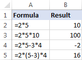
As shown in the screenshot below, Excel allow performing different arithmetic operations within one formula. Just remember about the order of calculations (PEMDAS): parentheses, exponentiation, multiplication or division whichever comes first, addition or subtraction whichever comes first.
How to multiply cells in Excel
To multiply two cells in Excel, use a multiplication formula like in the above example, but supply cell references instead of numbers. For example, to multiply the value in cell A2 by the value in B2, type this expression:
=A2*B2
To multiply multiple cells, include more cell references in the formula, separated by the multiplication sign. For example:
=A2*B2*C2

How to multiply columns in Excel
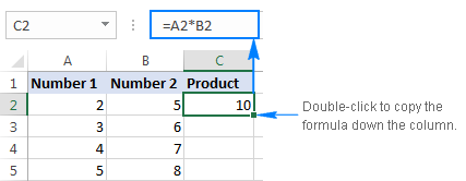
To multiply two columns in Excel, write the multiplication formula for the topmost cell, for example:
=A2*B2
After you've put the formula in the first cell (C2 in this example), double-click the small green square in the lower-right corner of the cell to copy the formula down the column, up to the last cell with data:
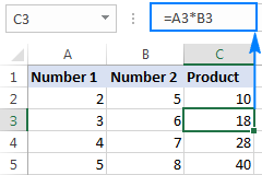
Due to the use of relative cell references (without the $ sign), our Excel multiply formula will adjust properly for each row:
In my opinion, this is the best but not the only way to multiply one column by another. You can learn other approaches in this tutorial: How to multiply columns in Excel.
How to multiply rows in Excel
Multiplying rows in Excel is a less common task, but there is a simple solution for it too. To multiply two rows in Excel, just do the following:
- Insert a multiplication formula in the first (leftmost) cell.
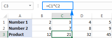
In this example, we multiply values in row 1 by the values in row 2, beginning with column B, so our formula goes as follows:
=B1*B2 - Select the formula cell, and hover the mouse cursor over a small square at the lower right-hand corner until it changes to a thick black cross.
- Drag that black cross rightward over the cells where you want to copy the formula.

As with multiplying columns, the relative cell references in the formula change based on a relative position of rows and columns, multiplying a value in row 1 by a value in row 2 in each column:
Multiply function in Excel (PRODUCT)
If you need to multiply multiple cells or ranges, the fastest method would be using the PRODUCT function:
Where number1, number2, etc. are numbers, cells or ranges that you want to multiply.
For example, to multiply values in cells A2, B2 and C2, use this formula:
=PRODUCT(A2:C2)
To multiply the numbers in cells A2 through C2, and then multiply the result by 3, use this one:
=PRODUCT(A2:C2,3)
The screenshot below shows these multiplication formulas in Excel:

How to multiply by percentage in Excel
To multiply percentages in Excel, do a multiplication formula in this way: type the equals sign, followed by the number or cell, followed by the multiply sign (*), followed by percentage.
In other words, make a formula similar to these:
- To multiply a number by percentage:
=50*10% - To multiply a cell by percentage:
=A1*10%
Instead of percentages, you can multiply by a corresponding decimal number. For example, knowing that 10 percent is 10 parts of a hundred (0.1), use the following expression to multiply 50 by 10%: =50*0.1
As shown in the screenshot below, all three expressions yield the same result:

How to multiply a column by a number in Excel
To multiply a column of numbers by the same number, proceed with these steps:
- Enter the number to multiply by in some cell, say in A2.
- Write a multiplication formula for the topmost cell in the column.
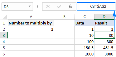
Assuming the numbers to be multiplied are in column C, beginning in row 2, you put the following formula in D2:
=C2*$A$2It is important that you lock the column and row coordinates of the cell with the number to multiply by to prevent the reference from changing when you copy the formula to other cells. For this, type the $ symbol before the column letter and row number to make an absolute reference ($A$2). Or, click on the reference and press the F4 key to change it to absolute.
- Double-click the fill handle in the formula cell (D2) to copy the formula down the column. Done!
As you can see in the screenshot below, C2 (relative reference) changes to C3 when the formula is copied to row 3, while $A$2 (absolute reference) remains unchanged:
If the design of your worksheet does not allow an additional cell to accommodate the number, you can supply it directly in the formula, e.g.: =C2*3
You can also use the Paste Special > Multiply feature to multiply a column by a constant number and get the results as values rather than formulas. Please check out this example for the detailed instructions.
How to multiply and sum in Excel
In situations when you need to multiply two columns or rows of numbers, and then add up the results of individual calculations, use the SUMPRODUCT function to multiply cells and sum products.
Supposing you have prices in column B, quantity in column C, and you want to calculate the total value of sales. In your math class, you'd multiply each Price/Qty. pair individually and add up the sub-totals.
In Microsoft Excel, all these calculations can be done with a single formula:
=SUMPRODUCT(B2:B5,C2:C5)
If you wish, you can check the result with this calculation:
=(B2*C2)+(B3*C3)+(B4*C4)+(B5*C5)
And make sure the SUMPRODUCT formula multiplies and sums perfectly:

Multiplication in array formulas
In case you want to multiply two columns of numbers, and then perform further calculations with the results, do multiplication within an array formula.
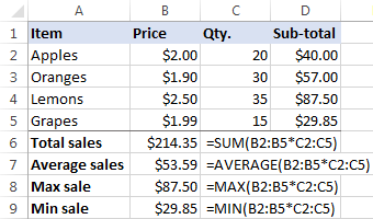
In the above data set, another way to calculate the total value of sales is this:
=SUM(B2:B5*C2:C5)
This Excel Sum Multiply formula is equivalent to SUMPRODUCT and returns exactly the same result (please see the screenshot below).
Taking the example further, let's find an average of sales. For this, just use the AVERAGE function instead of SUM:
=AVERAGE(B2:B5*C2:C5)
To find the largest and smallest sale, use the MAX and MIN functions, respectively:
=MAX(B2:B5*C2:C5)
=MIN(B2:B5*C2:C5)
To complete an array formula properly, be sure to press the Ctrl + Shift + Enter combination instead of Enter stroke. As soon as you do this, Excel will enclose the formula in {curly braces}, indicating it's an array formula.
The results might look something similar to this:
That's how you multiply in Excel, it doesn't take a rocket scientist to figure it out :) To have a closer look at the formulas discussed in this tutorial, feel free to download our sample Excel Multiplication workbook.
How to quickly do any calculations in Excel
If you are a novice to Excel and are not comfortable with multiplication formulas yet, our Ultimate Suite will make things a lot easier for you. Among 70+ cute features, it provides the Calculation tool that can perform all basic mathematic operations, including multiplication, in a mouse click. Let me show you how.
Supposing you have a list of net prices and you want to know the corresponding VAT amount. No big deal if you know how to calculate percentages in Excel. If you don't, have the Ultimate Suite do the job for you:
- Copy the prices to the VAT column. You need to do this because you don't want to override the original values in the Price column.
- Select the copied prices (C2:C5 in the screenshot below).
- Go to the Ablebits tools tab > Calculate group, and do the following:
- Select the percentage symbol (%) in the Operation box.
- Type the desired number in the Value box.
- Click the Calculate button.

That's all there is to it! You will have the percentages calculated in a heartbeat:

In a similar manner, you can multiply and divide, add and subtract, calculate percentages, and more. All you have to do is select an appropriate operator, for example the multiply symbol (*):

To perform one of the recent calculations to another range or column, just click the Apply Recent button, and pick the operation:

The results of all calculations done with the Ultimate Suite are values, not formulas. So, you are free to move or copy them to another sheet or workbook without worrying about updating formula references. The calculated values will remain intact even if move or delete the original numbers.
If you are curious to learn more about this and many other time-saving tools included with the Ultimate Suite for Excel, you are welcome to download 15-day trial version.
I thank you for reading and hope to see you on our blog next week!
 by
by
74 comments
Hi!
2X 12 1.22 1.22 0.15 2.68(Answer) Its Like this.
But I want Like this.
2X12 1.22 1.22 0.15 5.35(Answer)
Hi! Unfortunately, it is very difficult to guess what you want to do. I can assume that if you want to convert text into a formula, then this is possible using a VBA macro.
I Have a spread sheet that I would like to increase all of the values by 20% what is the formula please
Hello Bill!
Look for the example formulas here: Increase / decrease a number by percent.
Hi
I am trying to work out a percent of the total salaries for different departments, how do I do this please?
Thank you in advance
Hello Natasha!
If I understand your task correctly, this article may be helpful: How to calculate percentage in Excel - formula examples.
i want to multiply number of cells having value by a cell which has data validation list. So that whenver i change number in the list corresponding change should occur in all those cells which are linked to data validation cell
If Value is More than 40 need to Multiply with value and Column .How to enter in Excel
Hi! You can find the answer to your question in this article: IF function in Excel: formula examples for text, numbers, dates, blanks.
Hi! If I understand your task correctly, you can use in formulas an absolute reference to a cell that has a data validation list. The following tutorials should help: Relative and absolute cell reference: why use $ in Excel formula and How to copy formula in Excel with or without changing references.
How to calculate this?
H9*D12+D12*E12+F12
Hi! I recommend reading this guide: Basic Excel formulas & functions with examples.
Hallo,
Ben op zoek naar een formule die 3 cellen vermenigvuldigd, waarbij 1 cel regelmatig leeg is. Als de hele regel leeg is moet resultaat cel ook leeg blijven.
Hopelijk kunnen jullie me helpen.
Hi! You may find this article useful: Nested IF in Excel – formula with multiple conditions. To recommend a formula to you, give an example of source data and the desired result. Please do this in English.
Im trying to figure a way to calculate mileage distrubted. for Ex I have column A and it has 30 different millage ranges which all some up to Row (A31) 170,000. and the total budget is $20,000. I know how to get the average per mile which would be in row (A34) I put SUM(20,000/A31) and it gives me X
Now in column B I want to multiple each row by (A34) which looks like this =SUM (A1*A34) next is =SUM(A2*A34) but then I try to drag it down it keeps changing it to a different Cell From (A34). Can you help
Hi! To prevent the references from changing when copying, use absolute references in your formulas. For more information, read: Relative and absolute cell reference: why use $ in Excel formula.
Hi, can anyone help me with this formula I need to do a lot of them and it takes ages to do it manually but I don't know the quick way.
=SUMPRODUCT(J32*D32)+(J33*D33)+(J37*D37)+(J34*D34)+(J35*D35)+(J36*D36)+(J38*D38)+(J39*D39)+(J340*D40)+(J41*D41)+(J42*D42)+(J43*D43)+(J44*D44)+(J45*D45)+(J46*D46)+(J47*D47)+(J48*D48)+(J49*D49)+(J50*D50)+(J51*D51)+(J52*D52)+(J53*D53)+(J54*D54)+(J55*D55)+(J56*D56)+(J57*D57)+(J58*D58)+(J59*D59)
Thanks Becky
Hi! You can learn more about SUMPRODUCT function in Excel in this article on our blog.
=SUMPRODUCT(D32:D59,J32:J59)
how to calculate this? ( 0.89+0.88+0.87+0.87+0.86+0.86+0.85+0.85+0.84)*7.06 +(0.83+0.83+0.82+0.82+0.81+0.81+0.80+0.80+0.79+0.78+0.78+0.77+0.77+0.76+0.76+0.75)7.57 /(0.89+0.88+0.87+0.87+0.86+0.86+0.85+0.85+0.84+0.83+0.83+0.82+0.82+0.81+0.81+0.80+0.80+0.79+0.78+0.78+0.77+0.77+0.76+0.76+0.75) My ans. 59.53 but actual ans. 7.3765
My Formula = =SUM(F11:N11)*7.06+SUM(O11:AD11)*7.57/SUM(F11:AD11) Please help me with the right answer. thank you!
Hi! Perhaps you just need to remember the order of mathematical operations and add parentheses.
=(SUM(F11:N11)*7.06+SUM(O11:AD11)*7.57)/SUM(F11:AD11)
Hello! I would like to ask for some help with multiplying by a range of numbers. I should mention I'm not very good with math so I don't know all the terms, but what I'm trying to do is have a single column with a range of numbers (like 1 through 8) being multiplied. An example of a problem i'm trying to translate into excel would be:
4*(1-65%)*125
Hi!
In your formula, replace the number 1 with a reference to first cell of range. For example, 4*(A1-65%)*125.
Then copy that formula down the column.
I need to multiply three cells. first two cell has simple numbers but third cell has condition that
if number is <=99.99 then multiply by 1 and number above 99.99 multiply by 1.5 and add them both.
for example, if number is 112 then [(99.99*1)+(12.01*1.5)]*cell 1*cell 2
how do I write formula for this? TYA.
Hi!
If you have conditions then use the IF function
Try this formula:
=IF(A1 > 99.99,(99.99+(A1-99.99)*1.5)*B1*C1),A1)
I want to calculate the percentages of various amount like if i have 230,000 and 200,000 will get 0.5% and 30,000 will get 0.25%?
Please help... thanks...
Hello!
If you have multiple conditions, use the IF function as described in this article: Excel IF function with multiple conditions. I hope my advice will help you solve your task.
If Multiply using " =leftright "formula
150*150 in A1 Cell which is single cell
Let's have a look after applying formula in B1(reference cell is B1 where I want results
=LEFT(A1,3)*RIGHT(A1,3)
yes result is 22500 in b1,but what about I drag formula on down cell,if in next row A2 12*12 and formula automatically putted by draging but the result is" 0" it doesn't work cause chars or digit changed in A2 cell,if I change the formula manually in function bar =left(A2,2) replace 3 with 2, same way replace in=right( ,2) the result is 144
Exactly I need a single a formula which perform in any digits or chars,
Hi!
Determine the position of the "*" character using the SEARCH function. Extract the text to the right and left of this position using the substring functions.
=LEFT(A1,SEARCH("~*",A1)-1)*MID(A1,SEARCH("~*",A1)+1,20)
This should solve your task.
I have to calculate total number of days.
A1 cell has data 2.2.15 (ie.. 2 years.2 months,15 days)
Now, i want to convert this to total days with formula to calculate. And this formula to be applied for many cells
calculation = > 2*370+2*30+15=765 days.
Pl. share the formula to calcuate the same.
Hello!
To extract three values from text, you can use these three formulas:
=LEFT(A2, SEARCH(".",A2)-1)
=MID(A2, SEARCH(".", A2) + 1, SEARCH(".", A2, SEARCH(".", A2)+1) - SEARCH(".", A2)-1)
=RIGHT(A2,LEN(A2) - SEARCH(".", A2, SEARCH(".", A2,1)+1))
You can find the examples and detailed instructions here: Excel substring: how to extract text from cell.
To split text into cells, you can also use the Text To Columns feature.
Hi,
I'm struggling to find the right formula to multiply units by rates.
I have different materials with different units and rates. Rates are depend on quantities.
Description Unit Quantity Rate 1 Rate 2 Rate 4 Rate 5 Price
path m (QB) 50 11 13 13.5 14
road m (QB) 200
wall m2 (QB) 35
wood m 10
paint m2 12
Unit "Rate 1
(not exceeding)" "Rate 2
(not exceeding)" "Rate 3
(not exceeding)" "Rate4
(exceeding)"
day
h
m (QB) 10 50 200 200
m
m2 (QB) 10 50 150 15
m2
Hello how can I calculate cell 1*cell2 +cell3*cell4...../ 11?
Hi!
This is a complex solution that cannot be found with a single formula. If you have a specific question about the operation of a function or formula, I will try to answer it.
I have to know the excel formula for multiply more the three currency with one column
for e.g.
A
USD 100
B
AED 100
C
Eur 100
D
Exchange Rate
E
If the rate of USD is there I have to calculate with D exchange rate
If the value of C is AED is there then I have to Calculate with D exchange rate
How should I multiply this with excel formula?
Pls help
Hi!
If I understand you correctly, then in one cell D1 you want to write 3 exchange rate values. This is not possible in Excel. You can use the VLOOKUP function to select the desired exchange rate based on the currency. If there are a total of 3 exchange rates, write them down in separate cells (for example, F1:F3), and use nested IF function:
=IF(A1 < > "",F1,F(B1 < > "",F2,F(C1 < > "",F3,"")))
I hope it’ll be helpful.
INVOICE CURRENCY VALUE IN USD
USD INR AED EX RATE
$5,987.27 1.00 $-
Can excel complete a calculation for multiples of say 7. So you start obviously with 7, then have it auto generate out 14, 21, 28, 35, etc? And control its start and end number so if you wanted to start at say 336 and have it provide multiples of 7 generated out up to at least 1,000?
Hello!
You can create the sequence you want with the SEQUENCE function. See instructions and examples: How to make a date sequence in Excel with a formula.
I hope it’ll be helpful.
Hi,
How do I multiply a whole row by the same number?
Eg. All of row B needs to be multiplied by -1.
How would I do this
Thank you
Hi!
If you're talking about B, then it's a column, not a row. Please have a look at this article - How to multiply columns in Excel.
You can use this formula:
=D1:D13*(-1)
Hi,
How can I count a sum of multiple values where some have different percentage multipliers. E.g
A1:A1000 have different numeric values. The sum of these values is a percentage (eg. 60% x sum of values). BUT some specific values e.g. 89$ should be calculated with another percentage (70%.) How do I create a formula that calculates all values with 60% except 89 dollar values (with 70%) and adds them all up?
Hi!
To conditionally multiply, use SUMPRODUCT function:
=SUMPRODUCT(A2:A1000,IF(A2:A1000=89,0.7,0.6))
How do make the column multiply by itself without having to input the formula?
Hi!
This can be done with a VBA macro.