The tutorial shows how to combine VLOOKUP and IF function together to v-lookup with if condition in Excel. You will also learn how to use IF ISNA VLOOKUP formulas to replace #N/A errors with your own text, zero or blank cell.
Whilst the VLOOKUP and IF functions are useful on their own, together they deliver even more valuable experiences. This tutorial implies that you remember the syntax of the two functions well, otherwise you may want to brush up on your knowledge by following the above links.
Vlookup with If statement: return True/False, Yes/No, etc.
One of the most common scenarios when you combine If and Vlookup together is to compare the value returned by Vlookup with a sample value and return Yes / No or True / False as the result.
In most cases, the following generic formula would work nicely:
Translated in plain English, the formula instructs Excel to return True if Vlookup is true (i.e. equal to the specified value). If Vlookup is false (not equal to the specified value), the formula returns False.
Below you will a find a few real-life uses of this IF Vlookup formula.
Example 1. Look up a specific value
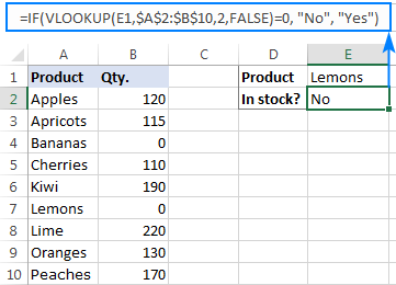
Let's say, you have a list of items in column A and quantity in column B. You are creating a dashboard for your users and need a formula that would check the quantity for an item in E1 and inform the user whether the item is in stock or sold out.
You pull the quantity with a regular Vlookup with exact match formula like this:
=VLOOKUP(E1,$A$2:$B$10,2,FALSE)
Then, write an IF statement that compares Vlookup's result with zero, and returns "No" if it is equal to 0, "Yes" otherwise:
=IF(VLOOKUP(E1,$A$2:$B$10,2,FALSE)=0,"No","Yes")

Instead of Yes/No, you can return TRUE/FALSE or In Stock/Sold out or any other two choices. For example:
=IF(VLOOKUP(E1,$A$2:$B$10,2)=0,"Sold out","In stock")
You can also compare the value returned by Vlookup with sample text. In this case, be sure to enclose a text string in quotation marks, like this:
=IF(VLOOKUP(E1,$A$2:$B$10,2)="sample text",TRUE,FALSE)
Example 2. Compare Vlookup result with another cell
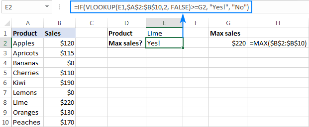
Another typical example of Vlookup with If condition in Excel is comparing the Vlookup output with a value in another cell. For example, we can check if it's greater than or equal to a number in cell G2:
=IF(VLOOKUP(E1,$A$2:$B$10,2)>=G2,"Yes!","No")
And here is our If formula with Vlookup in action:

In a similar fashion, you can use any other logical operator together with a cell reference in your Excel If Vlookup formula.
Example 3. Vlookup values in a shorter list
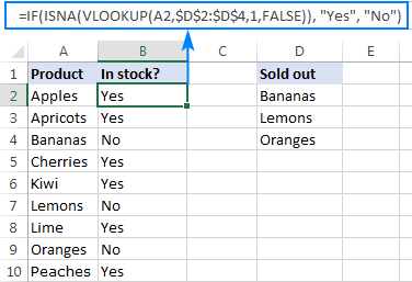
To compare each cell in the target column with another list and return True or Yes if a match is found, False or No otherwise, use this generic IF ISNA VLOOKUP formula:
If Vlookup results in the #N/A error, the formula returns "No", meaning the lookup value is not found in the lookup list. If the match is found, "Yes" is returned. For example:
=IF(ISNA(VLOOKUP(A2,$D$2:$D$4,1,FALSE)),"No","Yes")

If your business logic requires the opposite results, simply swap "Yes" and "No" to reverse the formula's logic:
=IF(ISNA(VLOOKUP(A2,$D$2:$D$4,1,FALSE)),"Yes","No")

Excel If Vlookup formula to perform different calculations
Besides displaying your own text messages, If function with Vlookup can perform different calculations based on the criteria you specify.
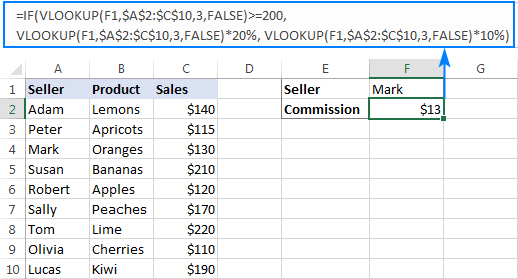
Taking our example further, let's calculate the commission of a specific seller (F1) depending on their effectiveness: 20% commission for those who made $200 and more, 10% for everyone else.
For this, you check if the value returned by Vlookup is greater than or equal to 200, and if it is, multiply it by 20%, otherwise by 10%:
=IF(VLOOKUP(F1,$A$2:$C$10,3,FALSE )>=200, VLOOKUP(F1,$A$2:$C$10,3,FALSE)*20%, VLOOKUP(F1,$A$2:$C$10,3,FALSE)*10%)
Where A2:A10 are seller names and C2:C10 are sales.

IF ISNA VLOOKUP to hide #N/A errors
If the VLOOKUP function cannot find a specified value, it throws an #N/A error. To catch that error and replace it with your own text, embed a Vlookup formula in the logical test of the IF function, like this:
Naturally, you can type any text you like instead of "Not found".
Supposing, you have a list of seller names in one column and sales amounts in another column. Your task is to pull a number corresponding to the name the user enters in F1. If the name is not found, display a message indicating so.
With the names in A2:A10 and amounts C2:C10, the task can be fulfilled with the following If Vlookup formula:
=IF(ISNA(VLOOKUP(F1,$A$2:$C$10,3,FALSE)), "Not found", VLOOKUP(F1,$A$2:$C$10,3,FALSE))
If the name is found, a corresponding sales amount is returned:

If the lookup value is not found, the Not found message appears instead of the #N/A error:

How this formula works
The formula's logic is very simple: you use the ISNA function to check Vlookup for #N/A errors. If an error occurs, ISNA returns TRUE, otherwise FALSE. The above values go to the logical test of the IF function, which does one of the following:
- If the logical test is TRUE (#N/A error), your message is displayed.
- If the logical test is FALSE (lookup value is found), Vlookup returns a match normally.
IFNA VLOOKUP in newer Excel versions
Beginning with Excel 2013, you can use the IFNA function instead of IF ISNA to catch and handle #N/A errors:
In our example, the formula would take the following shape:
=IFNA(VLOOKUP(F1,$A$2:$C$10,3, FALSE), "Not found")
Tip. If you'd like to trap all sorts of errors, not only #N/A, use VLOOKUP in combination with the IFERROR function. More details can be found here: IFERROR VLOOKUP in Excel.
Excel Vlookup: if not found return 0
When working with numerical values, you may want to return a zero when the lookup value is not found. To have it done, use the IF ISNA VLOOKUP formula discussed above with a little modification: instead of a text message, supply 0 in the value_if_true argument of the IF function:
In our sample table, the formula would go as follows:
=IF(ISNA(VLOOKUP(F2,$A$2:$C$10,3,FALSE)), 0, VLOOKUP(F2,$A$2:$C$10,3,FALSE))

In the recent versions of Excel 2016 and 2013, you can use the IFNA Vlookup combination again:
=IFNA(VLOOKUP(I2,$A$2:$C$10,3, FALSE), 0)
Excel Vlookup: if not found return blank cell
This is one more variation of the "Vlookup if then" statement: return nothing when the lookup value is not found. To do this, instruct your formula to return an empty string ("") instead of the #N/A error:
Below are a couple of complete formula examples:
For all Excel versions:
=IF(ISNA(VLOOKUP(F2,$A$2:$C$10,3,FALSE)), "", VLOOKUP(F2,$A$2:$C$10,3,FALSE))
For Excel 2016 and Excel 2013:
=IFNA(VLOOKUP(F2,$A$2:$C$10,3, FALSE), "")

If with Index Match - left vlookup with If condition
Experienced Excel users know that the VLOOKUP function is not the only way to do vertical lookup in Excel. The INDEX MATCH combination can also be used for this purpose and it's even more powerful and versatile. The good news is that Index Match can work together with IF in exactly the same way as Vlookup.
For example, you have order numbers in column A and seller names in column B. You are looking for a formula to pull the order number for a specific seller.
Vlookup cannot be used in this case because it cannot search from right to left. Index Match will work without a hitch as long as the lookup value is found in the lookup column. If not, a #N/A error will show up. To replace the standard error notation with your own text, nest Index Match inside IF ISNA:
=IF(ISNA(INDEX(A2:A10, MATCH(F1, $B$2:$B$10, 0))), "Not found", INDEX(A2:A10, MATCH(F1, $B$2:$B$10, 0)))
In Excel 2016 and 2016, you can use IFNA instead of IF ISNA to make the formula more compact:
=IFNA(INDEX(A2:A10, MATCH(F1, $B$2:$B$10, 0)), "Not found")

In a similar manner, you can use Index Match in other If formulas.
This is how you use Vlookup and IF statement together in Excel. To have a closer look at the formulas discussed in this tutorial, you are welcome to download our sample workbook below. I thank you for reading and hope to see you on our blog next week!
Practice workbook for download
Excel IF Vlookup - formula examples (.xlsx file)
 by
by
371 comments
i have required formula for below example
Month item code Required remark from formula
jan 1 exsting
jan 2 exsting
jan 3 exsting
jan 4 exsting
jan 5 exsting
jan 6 exsting
Feb 7 New for Feb
Feb 8 New for Feb
Feb 9 New for Feb
Feb 1 exsting
Feb 2 exsting
Feb 10 New for Feb
Feb 4 exsting
Hi,
Meanwhile I have also tried the below formula, and an Alert popped up reading "You've entered too few arguments for this function."
=IFERROR(IF(OR($I$16="Grimaldi Lines"),VLOOKUP(C20,Mapping_Product,8,FALSE),IF(OR($I$16="Normal Shipment"),VLOOKUP(C20,Mapping_Product,7,FALSE)," ")))
Appreciate your kind help.
Dear Svetlana,
I am currently using the below formula that works perfectly well. However, I need to eliminate #N/A in my empty cells.
=IF(OR($I$16="Grimaldi Lines"),VLOOKUP(C20,Mapping_Product,8,FALSE),IF(OR($I$16="Normal Shipment"),VLOOKUP(C20,Mapping_Product,7,FALSE)," "))
Whilst thanking you for anticipated kind and prompt attention, I look forward to hear from you.
Hi,
I Need to check 2 texts in 2 different columns, if both are in same row, then i want the row number. What would be the formula for that case?
Hello Giridhar!
If I understand your task correctly, please try the following formula:
=IF(A1=B1,ROW(),"")
I hope it’ll be helpful.
Hi Svetlana.. Thanks for this informative article as always.. I wanted to use dates as a criteria in vlookup.. for example I have some bills data and I want to lookup ex party sales value in suppose December to March period..How can we do that...
Thanks.
Hello Amit!
The VLOOKUP function can pull just one value from your table. If you need to count sales for a certain period of time, you have to sum a great number of bills to get the result. It means that VLOOKUP doesn’t suit for this task.
I recommend to use the SUMIFS function to get the sales result for several months.
Please see the detailed instructions on how to work with this function here: https://www.ablebits.com/office-addins-blog/excel-sumifs-multiple-criteria/
Hope this information will be helpful for you.
Hi, Having an issue with Vlookup returning an incorrect value
formula: =IF(VLOOKUP(A2,Sheet2!A:C,1,FALSE)=A2,Sheet2!B2,FALSE)
All the data is incorrect from the point of Jill in first sheet. It returned the figure associated with Pete (2nd sheet).
first sheet with results (formula is in local column)
global local first name
1 23 joe
3 45 jim
5 15 jack
7 300 jill
9 23 joanne
11 90 Joan
13 12 John
15 38 Jackie
17 75 Jorge
Sheet 2 that the data is being pulled from.
global local first name
1 23 joe
3 45 jim
5 15 jack
6 300 pete
7 23 jill
9 90 joanne
11 12 Joan
13 38 John
15 75 Jackie
17 83 Jorge
Can you help me fix this?
Hello,
Can anyone please help me with a search sheet formula that I have been trying to work on but haven't been successful?
I have a sheet that looks up from a big data of vehicle parts.
the criteria of my search is vehicle model, model year, part component and whether its genuine or oem or aftermarket. What I am looking for is the price which I have on a column.
Hi,
I need If and Vlookup logic together, but i should not get #NA error.
=IF(VLOOKUP(C5,$A:$B,2,0)=$O$2,"AB","PR")
In this case if the value in cell C5 is not in the range it's throwing #NA error. how to get it without that error.
=IF(VLOOKUP($E$10,$E$10:$E$12,1,0)="AC",IF(AND(F10>=0,F10$L$10,F10=0,F10$L$15,F10<$L$16),(F10-L15)*3+$M$15,0)))))))
Hi,
I have a H2 which has 10 in
In cell J2 i have 0 in
J2 Cell can change (sometimes it will be 0 sometimes it might be 15)
In cell k2 i need to calculate if j2 = 0 then leave blank however if j2 = more than 0 return whats in h2?
Can somebody help me please!
I need to use a formula to look up a value in a column (we'll call this #1), based on the value in another column (#2), and then finally return the value in the column to the left of #1 based on whether it not it matches a certain word. Would vlookup or index match work better?
=IF('20182019EmpSW'!$A$2:$A$122246="2019Ogos",VLOOKUP($A$5:$A$9000,'20182019EmpSW'!$B$2:$AA$122246,17,FALSE),VLOOKUP($A$5:$A$9000,'20182019EmpSW'!$B$2:$AA$122246,18,FALSE))
I'm trying to add an IF VLOOKUP with multiple search parameters - the idea I had was the following:
=IFERROR(VLOOKUP([@[LOCATION_NAME]],'SP Locations'!A:B,2,0)=No,VLOOKUP([@[LOCATION_NAME]],'SP Locations'!A:E,5,0)),
IFERROR(VLOOKUP([@[LOCATION_NAME]],'SP Locations'!A:B,2,0)=Yes,VLOOKUP([@[LOCATION_NAME]]&[@DEPTID],'SP Locations'!C:E,3,0))
I was wondering if it was at all possible to string the two IF searches together?
I need to return a text based on the result found in the VLOOKUP function on the other tab.
=IF(A2="","-",VLOOKUP(A2,'Current RP - RQTY (IMS)'!A$1:F$5000,5,FALSE))
If the following are found this is what I need returned to the cell... Can anyone help me out of the ditch on this one?
1 = RawMaterial
2 = Formula
3 = Container
4 = Substrate
Thank you in advance for any help you may have!!!
How to add vlookup along with below formula
=IFERROR(IF(AND(N5>$AN$2,N5<$AO$2),N5,"-"),0)
Can you tell me what is wrong with my formula? If my 'if statement' is true, I get the appropriate response of 62494, however, if my 'if statement' is false, my vlookup is giving me a #ref! error? UGH... helps if I include the function formula... sorry :) It's below:
=IF('Travel Expense Voucher'!$F$5=2,62494,VLOOKUP('Travel Expense Voucher'!M15,'Tcodes and Ecodes'!C11:D12,'Tcodes and Ecodes'!D11:D12,FALSE))
Can you tell me what is wrong with my formula? If my 'if statement' is true, I get the appropriate response of 62494, however, if my 'if statement' is false, my vlookup is giving me a #ref! error?
Sir/mam i need your help. I have a google sheet with of option chain data of multiple stocks. For each stock there are multiple strike prices. I need to get specific strike's premium when i put stock name in a cell. I tried to use IF and VLOOKUP together i got the results but the problem is,there are 70 stocks so i have to write the formula for each stocks that made it very very lenthy and time consuming. Please guide me. Thank you...
can this combination work for date formulas? i would like to create multiple formulas to find a list or sequence of dates to match any one person's payday. so that we dont have to rely on making a mistake on a paper calendar. so if someone gets paid weekly, bi weekly, semi monthly, on first of the month, or even on the 2nd, 3rd or 4th wednesday of the month.
I have three receipt date against one material code say X and in another excel file against material X i want to pick up latest date how can i do this
e.g.
material code - receipt date
X - 3-Sept-2019
X - 14-Aug-2019
X - 14-oct-2019
Now i want to pick up latest date i.e. 14-oct-2019 against material X
which formula to use
Please guide
Data is huge and in above case, i just gave you one sample.