VLOOKUP with IF statement in Excel

The tutorial shows how to combine VLOOKUP and IF function together to v-lookup with if condition in Excel. You will also learn how to use IF ISNA VLOOKUP formulas to replace #N/A errors with your own text, zero or blank cell.

Whilst the VLOOKUP and IF functions are useful on their own, together they deliver even more valuable experiences. This tutorial implies that you remember the syntax of the two functions well, otherwise you may want to brush up on your knowledge by following the above links.

Vlookup with If statement: return True/False, Yes/No, etc.

One of the most common scenarios when you combine If and Vlookup together is to compare the value returned by Vlookup with a sample value and return Yes / No or True / False as the result.

In most cases, the following generic formula would work nicely:

IF(VLOOKUP(…) = value, TRUE, FALSE)

Translated in plain English, the formula instructs Excel to return True if Vlookup is true (i.e. equal to the specified value). If Vlookup is false (not equal to the specified value), the formula returns False.

Below you will a find a few real-life uses of this IF Vlookup formula.

Example 1. Look up a specific value

Let's say, you have a list of items in column A and quantity in column B. You are creating a dashboard for your users and need a formula that would check the quantity for an item in E1 and inform the user whether the item is in stock or sold out.

You pull the quantity with a regular Vlookup with exact match formula like this:

=VLOOKUP(E1,$A$2:$B$10,2,FALSE)

Then, write an IF statement that compares Vlookup's result with zero, and returns "No" if it is equal to 0, "Yes" otherwise:

=IF(VLOOKUP(E1,$A$2:$B$10,2,FALSE)=0,"No","Yes")
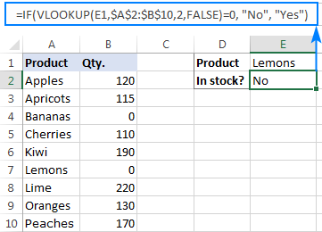
If Vlookup formula to return Yes or No based on vlookup result

Instead of Yes/No, you can return TRUE/FALSE or In Stock/Sold out or any other two choices. For example:

=IF(VLOOKUP(E1,$A$2:$B$10,2)=0,"Sold out","In stock")

You can also compare the value returned by Vlookup with sample text. In this case, be sure to enclose a text string in quotation marks, like this:

=IF(VLOOKUP(E1,$A$2:$B$10,2)="sample text",TRUE,FALSE)

Example 2. Compare Vlookup result with another cell

Another typical example of Vlookup with If condition in Excel is comparing the Vlookup output with a value in another cell. For example, we can check if it's greater than or equal to a number in cell G2:

=IF(VLOOKUP(E1,$A$2:$B$10,2)>=G2,"Yes!","No")

And here is our If formula with Vlookup in action:
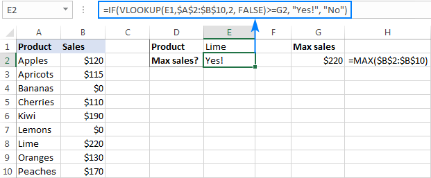
If formula with Vlookup to compare vlookup's result with another cell

In a similar fashion, you can use any other logical operator together with a cell reference in your Excel If Vlookup formula.

Example 3. Vlookup values in a shorter list

To compare each cell in the target column with another list and return True or Yes if a match is found, False or No otherwise, use this generic IF ISNA VLOOKUP formula:

IF(ISNA( VLOOKUP(…)),"No","Yes")

If Vlookup results in the #N/A error, the formula returns "No", meaning the lookup value is not found in the lookup list. If the match is found, "Yes" is returned. For example:

=IF(ISNA(VLOOKUP(A2,$D$2:$D$4,1,FALSE)),"No","Yes")
Vlookup values in a shorter list and return Yes or No.

If your business logic requires the opposite results, simply swap "Yes" and "No" to reverse the formula's logic:

=IF(ISNA(VLOOKUP(A2,$D$2:$D$4,1,FALSE)),"Yes","No")
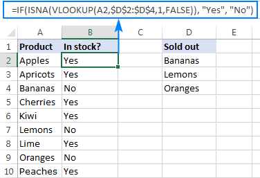
IF ISNA VLOOKUP formula to look up values in a shorter list and return Yes or No.

Excel If Vlookup formula to perform different calculations

Besides displaying your own text messages, If function with Vlookup can perform different calculations based on the criteria you specify.

Taking our example further, let's calculate the commission of a specific seller (F1) depending on their effectiveness: 20% commission for those who made $200 and more, 10% for everyone else.

For this, you check if the value returned by Vlookup is greater than or equal to 200, and if it is, multiply it by 20%, otherwise by 10%:

=IF(VLOOKUP(F1,$A$2:$C$10,3,FALSE )>=200, VLOOKUP(F1,$A$2:$C$10,3,FALSE)*20%, VLOOKUP(F1,$A$2:$C$10,3,FALSE)*10%)

Where A2:A10 are seller names and C2:C10 are sales.
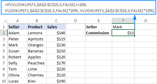
Excel If Vlookup formula to perform different calculations

IF ISNA VLOOKUP to hide #N/A errors

If the VLOOKUP function cannot find a specified value, it throws an #N/A error. To catch that error and replace it with your own text, embed a Vlookup formula in the logical test of the IF function, like this:

IF(ISNA(VLOOKUP(…)), "Not found", VLOOKUP(…))

Naturally, you can type any text you like instead of "Not found".

Supposing, you have a list of seller names in one column and sales amounts in another column. Your task is to pull a number corresponding to the name the user enters in F1. If the name is not found, display a message indicating so.

With the names in A2:A10 and amounts C2:C10, the task can be fulfilled with the following If Vlookup formula:

=IF(ISNA(VLOOKUP(F1,$A$2:$C$10,3,FALSE)), "Not found", VLOOKUP(F1,$A$2:$C$10,3,FALSE))

If the name is found, a corresponding sales amount is returned:
IF ISNA VLOOKUP formula pulls a matching value

If the lookup value is not found, the Not found message appears instead of the #N/A error:
If the lookup value is not found, IF ISNA VLOOKUP returns custom text instead of the N/A error.

How this formula works

The formula's logic is very simple: you use the ISNA function to check Vlookup for #N/A errors. If an error occurs, ISNA returns TRUE, otherwise FALSE. The above values go to the logical test of the IF function, which does one of the following:

  • If the logical test is TRUE (#N/A error), your message is displayed.
  • If the logical test is FALSE (lookup value is found), Vlookup returns a match normally.

IFNA VLOOKUP in newer Excel versions

Beginning with Excel 2013, you can use the IFNA function instead of IF ISNA to catch and handle #N/A errors:

IFNA(VLOOKUP(…), "Not found")

In our example, the formula would take the following shape:

=IFNA(VLOOKUP(F1,$A$2:$C$10,3, FALSE), "Not found")

Tip. If you'd like to trap all sorts of errors, not only #N/A, use VLOOKUP in combination with the IFERROR function. More details can be found here: IFERROR VLOOKUP in Excel.

Excel Vlookup: if not found return 0

When working with numerical values, you may want to return a zero when the lookup value is not found. To have it done, use the IF ISNA VLOOKUP formula discussed above with a little modification: instead of a text message, supply 0 in the value_if_true argument of the IF function:

IF(ISNA(VLOOKUP(…)), 0, VLOOKUP(…))

In our sample table, the formula would go as follows:

=IF(ISNA(VLOOKUP(F2,$A$2:$C$10,3,FALSE)), 0, VLOOKUP(F2,$A$2:$C$10,3,FALSE))
If Vlookup formula: if not found return 0

In the recent versions of Excel 2016 and 2013, you can use the IFNA Vlookup combination again:

=IFNA(VLOOKUP(I2,$A$2:$C$10,3, FALSE), 0)

Excel Vlookup: if not found return blank cell

This is one more variation of the "Vlookup if then" statement: return nothing when the lookup value is not found. To do this, instruct your formula to return an empty string ("") instead of the #N/A error:

IF(ISNA(VLOOKUP(…)), "", VLOOKUP(…))

Below are a couple of complete formula examples:

For all Excel versions:

=IF(ISNA(VLOOKUP(F2,$A$2:$C$10,3,FALSE)), "", VLOOKUP(F2,$A$2:$C$10,3,FALSE))

For Excel 2016 and Excel 2013:

=IFNA(VLOOKUP(F2,$A$2:$C$10,3, FALSE), "")
If Vlookup formula: if not found return blank (empty string)

If with Index Match - left vlookup with If condition

Experienced Excel users know that the VLOOKUP function is not the only way to do vertical lookup in Excel. The INDEX MATCH combination can also be used for this purpose and it's even more powerful and versatile. The good news is that Index Match can work together with IF in exactly the same way as Vlookup.

For example, you have order numbers in column A and seller names in column B. You are looking for a formula to pull the order number for a specific seller.

Vlookup cannot be used in this case because it cannot search from right to left. Index Match will work without a hitch as long as the lookup value is found in the lookup column. If not, a #N/A error will show up. To replace the standard error notation with your own text, nest Index Match inside IF ISNA:

=IF(ISNA(INDEX(A2:A10, MATCH(F1, $B$2:$B$10, 0))), "Not found", INDEX(A2:A10, MATCH(F1, $B$2:$B$10, 0)))

In Excel 2016 and 2016, you can use IFNA instead of IF ISNA to make the formula more compact:

=IFNA(INDEX(A2:A10, MATCH(F1, $B$2:$B$10, 0)), "Not found")
Using If with Index Match to do left lookup without N/A errors

In a similar manner, you can use Index Match in other If formulas.

This is how you use Vlookup and IF statement together in Excel. To have a closer look at the formulas discussed in this tutorial, you are welcome to download our sample workbook below. I thank you for reading and hope to see you on our blog next week!

Practice workbook for download

Excel IF Vlookup - formula examples (.xlsx file)

356 comments

  1. Hi!

    I'm wanting to first check a column to see if a person passes a level of cognitive ability before using VLookUp to determine their level of fit with the job. Specifically, if in column A it says "not fit" (meaning they didn't pass), I don't want to look at the rest of their scores (in another column) to determine their overall level of fit. How can I accomplish this? I feel like I need an If statement somewhere, but I don't know how to combine these together.

  2. Ive been following this thread with interest to find a solution to using vlookup based on a cell reference.

    Im trying to perform one of 3 vlookups within the same cell based on the value in a reference cell (ie: cell B3 contains either 1,2 or 3 which relates to data in a different sheet in the workbook) I then want to vlookup cell A3 in the corresponding sheet and return a value.

    My logic is =if B3=1 then vlookup A3 in sheet1 range A1:C100 and give me the value in column C else if B3=2 then lookup A3 in sheet2 same range and cell as before else if B3=3 then lookup A3 in sheet3 etc.

    Im struggling with correct format to perform the above so any tips are greatly appreciated.

  3. Hello team,
    Currently I am working on a table in which I have to do the following:
    1st Check if specific cell A1has writen "OK" and if it is true then return "4", If not then lookup another cell's value B1 and return a value from array C2:F8 corresponding to the previous cell B2.
    The tricky part is that in the array from the lookup there are blanks which must be bypassed. If C3 is blank then use C4, if C4 is blank then use C5 etc.
    =IFERROR(IF(A1="OK",4,VLOOKUP(B1,C2:F8,??????)),"ERROR")
    I am unsure how to implement ISBLANK or if there is another solution

    • Hello!
      And your explanation is not entirely clear what "corresponding to the previous cell B2" means. In addition, empty cells in the search column do not affect the result. Therefore, I don't really understand your problem. Maybe the VLOOKUP formula should be like this:

      =VLOOKUP(B1,C2:F8,B2,FALSE)

      If this is not what you wanted, please describe the problem in more detail.

  4. helped me a lot, thanks

  5. I want to make lookup and average at the same time.
    e.g.,
    "Sheet A" has data and time in one cell and i want to find that date and time exactly in "Sheet B".
    Once i find in "Sheet B" the exact date and time in next column i want to have average of last 15 values or cells. And this all i need to see in sheet one with 15 cell average.

    Please assist urgent.

    • Hi!
      Unfortunately, your task cannot be solved using single Excel formula. I can't see your data, but I think you should use a VBA macro.

  6. Hello Team :)
    I am trying to to use the IF function with a lookup table, using a value of 1 for males, 2 for females, to search and return the correct result depending on which gender applies.

    My current, formula is:

    =IF(C2=1,VLOOKUP(C2,B25:E30,2),VLOOKUP(C2,B25:E30,3))*1000

    The formulas for each age group are in two colums, column 3 for males, column 4 for females.
    I can't get the formula to choose the right column as designated by the 1 or 2 choice.

    I'm not sure if that is sufficient information.

    Additional information:

    Using Schofield's formula to calculate daily (basal) energy needs

    SCHOFIELD BMR EQUATION - MEGAJOULES

    AGE GROUP WEIGHT MEN WOMEN

    10 - 18 83 8.896 7.546
    19 - 30 83 8.125 7.182
    31 -60 83 7.637 6.360
    > 60 83 6.526 5.909

    A person over 60 weighing 83kg needs 6.526 mj (males) or 5.909 mJ (females).

    I just need to lookup to to choose according to the 1 or 2 designated - 1 will return 6.526, 2 will retun 5.909.

    Thanks!

    • Hello!
      If I understand your task correctly, the following formula should work for you:

      =IF(C2=1,VLOOKUP(C1,B25:E28,3,TRUE),VLOOKUP(C1,B25:E28,4,TRUE))

      C2 is 1 or 2
      C1 - this is the age in years.
      B25:B28 is 10, 19, 31, 60

      Read about VLOOKUP approximate match (TRUE) in this article.
      This should solve your task.

  7. can u help me with this scenario

    final numerical
    performance rating
    8.38 <-------------RATING BUT IT DISPLAY (VS)
    equivalent adjectival rating
    = (VS) <------ I WANT TO SHOW SOMETHING LIKETHIS
    THE DATA BELOW RANGE FROM
    9.5-10 = OUTSTANDING (O)
    7.51-9.49= VERY SATISFACTORY (VS)

    THANKS

  8. Hi,

    Have a peculiar query.

    The following table denotes achieve numbers in the unit tests.
    Name Unit 1 Unit 2
    A 100
    B 95 98
    C 85
    D 92 96
    E 65 85
    F 99
    G 85 92

    Whosoever have taken UNIT 2 test. That number will be considered, else UNIT 1 number.

    Pls help with formula

  9. I have the almost the same data with example number 1 but instead of it being zero (0), the column is blank (no data). How do I replace the (0) in the formula if the data in the column is empty?

    =IF(VLOOKUP(E1,$A$2:$B$10,2,FALSE)=0(what if the value of column is empty/no data?),"No","Yes")

  10. Hi,

    I need help with a formula. I need to do a Vlookup or formula based on a location I type in the cell to reference that locations data. If I type a location in a cell (ex. Atlanta) I need to do a Vlookup based on location 1's (Atlanta's) data. If I enter location 2 (ex. Charlotte) in the cell I need to reference location 2's (Charlotte's) data.

    Thank you,

    • Hello!
      Unfortunately, without seeing your data it is difficult to give you any advice. If you enter location data in cell A2, then in the formula in cell B2 you must use the data from A2. You can see examples of VLOOKUP in this article.
      If this is not what you wanted, please describe the problem in more detail.

    • Correct me if I'm wrong

      based on my understanding @hollie has 2 different set of data which are known as Atlanta and Charlotte as separate table and @hollie want to use those data set as vlookup point of refference for return value

      I'm still learning and advice my solution since I just get the undertanding of the formula 2 minutes ago

      Hollie need to combine Charlotte and Atlanta Table as one big table and ensure to use unique data as first column also using those unique value as data entry for serching return value

  11. Please help!
    I have a template that I'm using a vlookup to populate the dollar value for the salary range's minimum, midpoint, and maximum. However, in the lookup table, if the job code doesn't have a salary range, the value appears as "1" for the minimum, midpoint, and maximum.

    I'd like the vlookup to return the value shown for the minimum, midpoint, and maximum, unless it equals "1", then I want it to displayed value to show "N/A" in the template.

    The following formula is correct, except it's missing the value shown in the lookup table when the value is greater than 1.

    =IF(VLOOKUP($F$9,'Active Job Codes List (25)'!$A$2:$Z$4168,14,FALSE)=1,"N/A")

    The following formula is correct, except it's missing the "N/A" if the value shown in the lookup table equals 1.

    =VLOOKUP($F$9,'Active Job Codes List (25)'!$A$2:$Z$4168,14,FALSE)

    Basically, I need to combine these two formulas and none of the options I've tried seem to work.

    Thank you!

    • Hello!
      Based on your description, it is hard to completely understand your task. However, I’ll try to guess and offer you the following formula:

      =IF(VLOOKUP($F$9,’Active Job Codes List (25)’!$A$2:$Z$4168,14,FALSE)=1,”N/A”, VLOOKUP($F$9,’Active Job Codes List (25)’!$A$2:$Z$4168,14,FALSE))

      If this is not what you wanted, please describe the problem in more detail.

  12. I'm trying to do a lookup formula that if true will display "present" but if false, will look in another sheet to find a "present" mark. Is this possible?

    So if J Bloggs was absent on Monday's sheet returning "absent", but did attend on Tuesday's sheet, I want the tuesday's sheet mark to return so it is clear to see if anyone hasn't attended that week.

  13. Hello,=IF(HLOOKUP(J17,shopdirection,4,0)="L17","Y","N"),he output is either all yes or all No,why

    • Hello!
      I can't see your data and I don't know what your formula should do. Try removing the quotes.

      =IF(HLOOKUP(J17,shopdirection,4,0)=L17,”Y”,”N”)

  14. Hi I am looking to subtract one lookup to the other.
    =(vlookup(T11,A7:H155,4,false))-vlookup(T11,M12:R80,5,false)

    But if the cell for the second lookup value is empty, i would like it to just display the first value. How to I go about doing that?

    Thank you!

  15. Hi! I am trying to write a formula that compares names across two different excel sheets. With that being said I wrote a formula that takes the value for a month (say August) and subtracts it from a prior month (July). The three values it can return are -1 , 0 , and 1. I only care when the resulting figure is a 1. Here is the formula I have so far:

    =IF('TB VI 2021.09.10'!E10-'TB VI 2021.07.31'!E10=1,1,IF('TB VI 2021.09.10'!E10-'TB VI 2021.07.31'!E10=0,"",IF('TB VI 2021.09.10'!E10-'TB VI 2021.07.31'!E10=-1,"",)))

    However, it is important that the formula pulls data from the correct names in August and in July. Sometimes, a name appears in a different cell spot across each month. I need to add something to this formula that takes the value from a specific name in one month (August) and finds that name in another month (July) and performs the subtraction (above formula)

    Let me know if this is feasible or I can elaborate any further

    • Hello!
      Please check out this article to learn how to search multiple sheets using VLOOKUP.
      I hope my advice will help you solve your task. If something is still unclear, please feel free to ask.

      • Help me to this problem

        1=8
        2=22
        3=40
        4=62
        5=86

        I WANT THE CODE TO DO THIS

        1.5=(value of 2 minus value of 1) "the answer is 14"
        14x.5 " decimal point of 1.5"
        Answer is 7
        7+value of 1
        answer is 7+8=15

  16. Hello I need help with a formula
    I need to extract details available in one column to a specific format.
    Attached please find the format, if anyone can help would be really helpful.

    Details I get in a column is:

    Roll Number:123456 House Number:789654 Last Name: rfhdfsdf Address: asdasfSFSFLKHKGKLHG

    I need a formula to extract it in below format to avoid manual task

    Roll Number
    House Number:
    Address:

    Why I am stuck is,

    1. the length of roll numbers and house numbers would change from a single digit to double or triple
    2. I do not want to extract last name as per the format, hence not able to use mid/left/right formula

    • Hello!
      If I understood the problem correctly, you can extract the last name from the text using the formula:

      =MID(REPLACE(A1,1,SEARCH("Last Name:",A1)+11,""),1, SEARCH(" ",REPLACE(A1,1,SEARCH("Last Name:",A1)+11,""))-1)

      • Thanks for your response Alex.

        No, the problem is I get below details in one cell "A2"

        Roll Number:123456 House Number:789654 Last Name: rfhdfsdf Address: asdasfSFSFLKHKGKLHG

        I have a different excel sheet, wherein I need to extract only Roll Number, House Number & Address from the cell manually, to different different columns of another excel sheet.

        Therefore need a formula.

        • Hi!
          I wrote a formula to extract the last name. Replace "Last Name:" with "Address" in the formula and you will get the address.

          • Great thanks Alex, it was resolved partly by getting the Roll Number and House number & Last name for me.
            But for House number Somehow not getting results for address. I tried changing the number from 11 to 7,8 - 13 and so on - considering the same logic by adding the number of character it has.

            Just help with this now and it will be resolved completely. Anyways a big thanks, it was such a great help!

            Sorry for the long chain of comments.

            • Sorry read it as not getting results for Address
              Rest all sorted
              Sorry for Spamming

              • I was making some idiotic mistake
                It has completed resolved
                Thanks for offering this platform sir
                And really sorry for the long chain. Actually I was really pissed off this manual task and was very overwhelmed when I got to learn about this platform in order to get some insights.

                Thank you so much!

  17. Hi Mr. Alexander, thank you so much because of you I learned a lot of things you also helped me before when I struggle searching for the right formula, I am new in Vlookup actually I started learning about it today, Im having trouble with this scenario, I wish to auto populate data in my table but there are so many criteria and range to consider I have column A for terms such as 12 mos,24 mos,36 mos each month have corresponding value for column B standard rate and column C advanced rate(I made it in dropdown list). I wish to autopopulate (column c row 6) the corresponding value when I input the term and whether I choose the standard rate or advance rate

    A - B - C
    mos - standard rate -advance rate
    12 - 1% - 4%
    24 - 2% - 5%
    36 - 3% -6%

    row 5 | mos - 24
    row 6| rate - standard rate (in dropdown form) |column C 2%

    I was able to do this but the problem is I can only choose to look for the data for standard rate I wish that even if I change from standard to advance it will automatically auto populate

    I hope you understand my concern Thank you

    • Hello!
      Write down the formula to find advance rate versus standard rate in column C. Write down the formula to find standard rate versus advance rate in column B. If you write a value in column B or C, you will replace the formula with a value. But the formula in the adjacent column will find the value you want.
      I hope my advice will help you solve your task.

  18. Hi,

    I am trying to get the below formula to work. I don't know what I am getting wrong over here. Can someone please help with the same.

    =IFS(M3="",O3,O3="",R3),IFNA(VLOOKUP(M3,'Sponsor List Ref'!B2:C95,2,0),VLOOKUP(M3,'Sponsor List Ref'!$F$2:$G$6,2,0)))

    The formula works well with only IFNA part, but if i add the IFS before, it gives a #Value! error. Any input is appreciated.

    Thanks.

    • Hi!
      The formula you wrote cannot be entered into a cell. Incorrect syntax. I don't know what you want to count. Formula =IFS(M3=””,O3,O3=””,R3) is complete. If you need to add the condition into it -

      =IFS(M3=””,O3,O3=””,R3, logical_test3, value_if_true3)

      Check out the syntax for the IFS function in this tutorial.

  19. Hello,

    Scenario - we have to collect the timestamps for using some badges: the entrance usage (IN) and the exit usage (OUT). One badge can be used multiple times (of course, after it has closed the cycle - exit/OUT).

    I have 2 sources where i store the badge ID and a timestamp used: one sheet with the entrance - badge ID, timestamp_IN, the other with the exit - badge ID, timestamp_OUT.

    How can i return for the same line the value timestamp_OUT based on the badge ID that was used before (timestamp_IN) ? Trying with VLOOKUP, but it obviously returns the first date. I need to insert a condition that the imestamp_OUT must be > than the timestamp_IN for the current line....

    in sheet_IN we have the following records (badge | timestamp_IN )
    badge1 | 2021-09-16 08:20:35
    badge2 | 2021-09-16 08:25:44
    badge3 | 2021-09-16 08:31:10
    badge3 | 2021-09-16 09:00:30
    badge1 | 2021-09-16 09:08:12
    badge2 | 2021-09-16 10:44:03

    in sheet_OUT we have the following records (badge | timestamp_OUT )
    badge1 | 2021-09-16 08:28:15
    badge3 | 2021-09-16 08:58:37
    badge1 | 2021-09-16 09:02:40
    badge2 | 2021-09-16 10:12:03
    badge3 | 2021-09-16 11:07:17
    badge2 | 2021-09-16 12:32:53

    How to get the proper values from sheet_OUT from each badge so we know the timestamp_IN and timestamp_OUT on the same line (either in the first sheet - sheet_IN or in a new one)?

    The result should contains the following records:

    badge | timestamp_IN | timestamp_OUT

    badge1 | 2021-09-16 08:20:35 | 2021-09-16 08:28:15
    badge2 | 2021-09-16 08:25:44 | 2021-09-16 10:12:03
    badge3 | 2021-09-16 08:31:10 | 2021-09-16 08:58:37
    badge3 | 2021-09-16 09:00:30 | 2021-09-16 11:07:17
    badge1 | 2021-09-16 09:08:12 | 2021-09-16 09:02:40
    badge2 | 2021-09-16 10:44:03 | 2021-09-16 12:32:53

    Thank you all!

  20. I'm trying to create a template spreadsheet that always has VLOOKUP in Column C, going down 10,000 rows. This will check to see if the value in a specific cell in Column A is present in any of Column B, and returns "Yes" or "No" depending on the information. All good there.
    Sometimes I don't need all 10,000 rows, sometimes I do, but I don't want to change the template for this VLOOKUP. If I only have 50 rows with data in both Column A and Column B, I want Column C to be blank in every cell below C50 instead of returning a "no" result. This way when I filter Column C to only see the "no" cells it doesn't show all the results below C50 as well.
    For Visual:
    A B C
    1| Hello | Hello | Yes |
    2| Hi | Wave | No |
    3| 'blank'| Apple |'stays blank' |
    Currently I'm stuck on:
    =IF(ISNA(VLOOKUP(A1,$B$1:$B$10000,1,FALSE)),"No","Yes")

    • Hello!
      Use the IF function to get blank if the cell in column A is blank.

      =IF(A1<>"",IF(ISNA(VLOOKUP(A1,$B$1:$B$10000,1,FALSE)),"No","Yes"),"")

      Hope this is what you need.

      • Right on the money! Thank you for getting me out of that rabbit hole!

  21. Hi I want to do a vlookup of a cell that ends with N with multiple results
    Sample:
    Apple 13A
    Banana 76
    Mango 57S
    Apple 26N

    I want to vlookup apple with the result of 26N because it ends with "N". Please help me

  22. I am not understanding whatever you are saying?

    explain in detail.......

  23. Hi Alexander I have a formula I need help with.

    =@IF(VLOKUP(@I:I,Format2!C:P,14,0)="Scrunchie","Marketing Merchandise",AE:AE)

    Would like to add in Bottle Holder and Mask besides scrunchie , total 3 items to the formula to show Marketing Merchandise as the result.

    Hope to hear a reply from u soon !

    Thanks!

  24. Hi, I have a billing template, I have 3 areas with the same item # and one of them has a different price. In the tracker, I need a formula that if I use the same code for the different areas, the formula gives me a different price for each area. For example, I have 82 feet of item# LC04 for Tampa with a cost of $5.82 per foot and the same item with the same footage for Lakeland with a cost of $6.59. What formula do I use to calculate the value? I already have the tab for the items and another tab for the billing. Please help??

  25. Hi there,
    I would like to use google sheets to do the following production planning. It is a two part plan.

    1) I would like to be able to write on the left the following information in cells A1:D7 for example

    Brew Date Batch Number FV No. F. Time
    07/06/2021 RF130 FV1 20
    08/06/2021 RF131 FV2 16
    09/06/2021 RF132 FV3 14
    10/06/2021 RF133 FV4 16
    11/06/2021 RF134 FV5 30
    12/06/2021 RF135 FV6 20

    I would then like to automatically populate a schedule that has the days running down it and the fermenter number across with the batch number ie
    FV1 FV2 FV3 FV4 FV5 FV6 FV7 FV8 FV9
    07/06/2021 RF130
    08/06/2021
    09/06/2021
    10/06/2021
    11/06/2021
    12/06/2021
    13/06/2021

    my current formula returning RF130 is a simple IF(AND but I have to enter a million IF and statements as I run down the page
    =
    IF(AND(A2=F4,C2=G3),B2,IF(AND(A3=F4,C3=G3),B3,IF(AND(A4=F4,C4=G3),B4,IF(AND(A5=F4,C5=G3),B5,
    IF(AND(A6=F4,C6=G3),B6,IF(AND(A7=F4,C7=G3),B7,IF(AND(A8=F4,C8=G3),B8,""))))))). etc

    I would like to migrate to a formula that matches date and FV number and returns the batch number for the specified FV.

    2) The second part of the formula will look at the F.Time and populate down the same batch number for that amount of days.
    please help!
    cheers
    G

  26. Hi

    I have list of DMAs for which I need to vlookup states (col 2) but pick only which has max vehicle count in (col 3).
    what formula would you recommend?

    DMA State Vehicle Count
    ALBANY MA 2,272
    ALBANY NY 26,361
    ALBANY VT 830
    SANTA FE. AZ 1,033
    SANTA FE. CO 1,132
    SANTA FE. NM 26,917

  27. If i want to apply vlookup formula and want to make difference two reference column how can I did it.

  28. Hi Alexander,

    I am looking for a formula that looks like a combination of Vlookup and IF function.
    following is my scenario:

    TAB 1 contains data of numbers negatives to positive, i want to reflect that data to TAB 2 with the condition , if value is less than zero like negative no. then return it as Zero "0" and if above zero then return as it is.

    Thank you so much,

    • I think i found it , please disregards my question above, thank you

      Excel If Vlookup formula to perform different calculations
      Besides displaying your own text messages, If function with Vlookup can perform different calculations based on the criteria you specify.

      Taking our example further, let's calculate the commission of a specific seller (F1) depending on their effectiveness: 20% commission for those who made $200 and more, 10% for everyone else.

      For this, you check if the value returned by Vlookup is greater than or equal to 200, and if it is, multiply it by 20%, otherwise by 10%:

      =IF(VLOOKUP(F1,$A$2:$C$10,3,FALSE )>=200, VLOOKUP(F1,$A$2:$C$10,3,FALSE)*20%, VLOOKUP(F1,$A$2:$C$10,3,FALSE)*10%)

      This will do, any number multiply zero will equal to zero.

    • Hello!
      Please try the following formula:

      =IF(Sheet1!A1>0,Sheet1!A1,0)

      You can copy this formula down along the column.
      Hope this is what you need.

  29. I am looking up a specific value from two tables I set up, one table has one rate, another has a different rate. I am using IF (VLOOKUP, true), (VLOOKUP2, true), false). How do I make the VLOOKUP2 value work? Thanks!

    • Hello!
      Please specify what you were trying to find, what formula you used and what problem or error occurred. Include an example of the source data and the result you want to get. It’ll help me understand the problem you faced better and help you.

      • Thank you Alexander!

        Here is the formula I am trying to make work:

        Rule: if Column J is in TableFX25 then Column I* (1-0.025), if column J is in TableFX35, ColumnI*(1-0.035) else Column I*(1-0.03).

        The fomula: N8*IF(J8 =(VLOOKUP(J8,'FX Calculation.xlsx'!TableFX25,1,FALSE)),(1-0.025),IF(J8=(VLOOKUP(J8,'FX Calculation.xlsx'!TableFX35,1,FALSE)), (1-0.035), (1-0.03)))

        Problem: Vlookup for TableFX35 isn't working - the value in column J isn't being recognized in TableFX35.

        Is it because the formula?

        Appreciate the help. And let me know should you need further clarification.

        • Hello!
          Use the IFERROR function.
          Instead

          J8 =(VLOOKUP(J8,’FX Calculation.xlsx’!TableFX25,1,FALSE))

          write down

          J8 =IFERROR(VLOOKUP(J8,’FX Calculation.xlsx’!TableFX25,1,FALSE),"")

          You can learn more about IFERROR function in Excel in this article on our blog.

  30. I am comparing two cells (contains nos.) which have Vlookup formula in it by simple IF formula.
    My logical test value is true but it is still not showing the desired result and showing the text of false value.

    Where I am going wrong?

    • Hi!
      The information you provided is not enough to understand your case and give you any advice. If the numbers are the result of formula calculations, check the decimal places. Perhaps your numbers differ by the third or fourth digit after the decimal point. Use rounding of results in formulas.

  31. i need function calculate variable discount for different products
    with if and & vlookup

  32. trying to write a vlookup with where if is a certain cell i would like it to multiply to the power of 10 and than divide by 2 and if it is not the certain cell than to just multiply by power of 10 here is what i got so far.

    =IF(OR(E2="",$D2=""),"",SUM(IF($C2="Buy",(E2-D2),(D2-E2)) * POWER(10, VLOOKUP($L2,'Pairs time power of 10'!$A:$C,3,FALSE)),0))

    I need to add this

    IF(b2 is 'Pairs time power of 10'!B37,'Trading Journal'!, divide by 2

    I hope i explained what im looking for correctly. the equation i have already is perfect for my other pairs for forex, but a few are stubborn and need to be divided by 2, so i am trying to figure it into the equation

  33. Hey,

    I have following issue.

    for example my If should be: if the content of cel from kolom A on this row occurs in kolom B then it should say "Slave" else it should say "Master"

    We used this formule: =IF(VLOOKUP([@[xxx]]=@xxx_HP;1;FALSE)=TRUE;"Master";"Slave")
    But we get a #N/A

    Thanks

    • Hi,
      It is very difficult to understand a formula that contains unique references to your workbook worksheets.
      Explain what xxx and xxx_HP are.
      Describe in detail what problem you have, and I will try to help you.

  34. Hello,

    I am trying to lookup 3 criteria's from a range of data on a different sheet, and match to 3 criteria's on my current sheet and if they all match say "Yes", if Not say "No".

    Can you please help me with that.

    Thanks

    • Hello!
      Please re-check the article above since it covers your task.
      I cannot give more detailed advice, since I do not have your data. If something is still unclear, please feel free to ask.

  35. good day, I want to extract information out of an excel table for every customer that needs a refund. i made a column that states "REFUND DUE" and it says "yes" or "no" for when refund is or isnt due. i need to extract all the "yes" to another table. what formula can i use to do so?

  36. Hi :)
    I have a unbalanced panel data set I want to sort.

    How can I code excel to look in a column match with a condition, and then take the sum of the values which also meets the same condition?

    The goal is to get the mean of my parameter for each country for each year in the panel data set. So I only have the parameter in years for each country.

    I was thinking that some of the functions here could be usefull, but I cant quite figure out how to combine them to get the wanted result.

  37. I have two sheets. In the first sheet I miss a date, which can be found in the second sheet. The rows (in the second sheet) in which these dates can be found is also a unique ID. These ID numbers are also present in the rows in the first sheet which requires the dates.
    I would like to define a formula that takes the dates from the second sheet and prints it in the right cell in the first sheet. The date is placed correct if the ID in the first and second sheet match.

    How can I use 'IF' and 'VLOOKUP' to define such a formula?

  38. I have a data in which The team mapping from 1st-24th was different and then from 25th the team mapping has changed how can I use the If with Vlookup

  39. is there a way to show vlookup result in series? vlookup always show first value
    for example:
    order number 1 has to 2 order item1 apple item 2 is orange item3 is banana

    order # | item
    1 apple
    1 apple
    1 apple

    instead of:
    order # | item
    1 apple
    1 orange
    1 banana

    please help me on this
    thanks!

  40. I'm trying to match information from two sheets (First Name, Last Name & DOB), but also need the formula to pull data from 3 separate columns if a match is found (Date, Action, Customer ID).

    Sheet 1 only has First Name, Last Name & DOB.
    Sheet 2 has First Name, Last Name & DOB + a specific date, an action (Add or Delete) and a customer ID.

    Can this be done with IF+VLOOKUP?

    Thanks!

  41. Hoping for your best formula by understanding what I want the outcome is.

    My situation is like this. In cell H4 and I4 is the Basic Pay on an employee separated whether the basic is MWE or not, so only one cell will only have the data needed. In cell AD4 is the EE share for PHIC here in Philippines. In cell AR4 should be the ER share (this is where I want my formula to work on).

    In another sheet 'Formula Source'!B2:E5 is my table range where my vlookup should return the value in index 3 (or in any value in Cell D2 to D5). But the value in D2 is a fix amount of P300 and in D3:D5 is only a percentage rate given with a compensation range in B2:B5.

    My formula goes like this: =IF(OR(SUM($H4:$I4)>'Formula Source'!$B$3,$AD4>0),(SUM($H4:$I4)*VLOOKUP(SUM($H4:$I4),'Formula Source'!$B$3:$E$5,3,TRUE)),VLOOKUP(SUM($H4:$I4),'Formula Source'!$B$2:$E$2,3,TRUE))

    Well, this gave me a result but even those who are zeros in AD4 (column AD) still have values where this should also be zero.

    Hoping for your better analysis. Thank you.

    • Compensation range is actually in B2:C5

    • Hello!
      It is very difficult to understand a formula that contains unique references to your workbook worksheets.
      I don't know anything about how salaries are calculated in the Philippines. Therefore, your abbreviations MWE, PHIC, ER do not tell me anything.
      Describe your problem more easily.

  42. Please help here to find a match value, which formula should I use to get it. Example below.

    In Column A I have a value and on that basis I need to find a match with reference to the Multiple column like, if you find a match for column A from column B give me a value if not find in Column B look in column C and if not column C look in column D and give me a value.

    Which formula should I use here. Thanks.

  43. I have a worksheet with two tabs. My first tab (A) is my results page and I usually use a vlookup to match identifiers from Tab A to Tab B that then finds associated data for the identifier. (eg: (VLOOKUP(B4,'INFO_201801-201812'!G:H,2,FALSE) That is usually fine, as the data I need is always in a specific place on my Tab B. However, I have found an issue with my original data and the identifer in Tab B can be found in one of two different columns. (eg: F:H or G:H) Can i combined two vlookup formulas into one IF statement so that, if the data I need is not found in the first column (F) on Tab B it will check the second column (G)?

    • Hello!
      Pay attention to the following paragraph of the article above — ISNA VLOOKUP.
      Try something like this.

      =IF(ISNA(VLOOKUP(F1,Sheet1!$A$2:$C$10,3,FALSE)), VLOOKUP(F1,Sheet2!$A$2:$C$10,3,FALSE), "Not found")

      Modify the links according to your details.

  44. I am looking for a formulas that I am guessing is some sort of IF and VLOOKUP combination.
    I have a Main excel sheet that will hold all "donations" made: Name, contact info and a column of each department a donation was made to.
    Each Department has it's own column and its own sheets, so I would like Names and contact Infor & amount donated shared with that departments sheet, if there is an amount in the main sheets column.
    So IF Column4 has $ammount in Row1, Then Name, address, phone #, email, and $amount in Row1 is shared with the corresponding Sheet for Column4.

    • Hello!
      Unfortunately, without seeing your data it is impossible to give you advice.
      I'm sorry, it is not very clear what result you want to get. Could you please describe your task in more detail and send us a small sample workbook with the source data and expected result to support@ablebits.com? Please shorten your tables to 10-20 rows/columns and include the link to your blog comment.
      We'll look into your task and try to help.

  45. Hi,

    I have an other problem (I think).

    I do a VLookup. But if the cell of the requested Output is empty, I want to get the next value (lookup the next row in the range that equals the Lookup match.

  46. So I am have question and I am not sure if it can be done with excel.
    I have 3 columns, I am comparing the data from columns A and B using VLOOKUP
    to express the results on column C, I get the result of N/A for the values missing from
    A and B. Is there a way instead of showing 'N/A' to show the values from column A
    so I know exactly which values are not present in Column B? I don't want to see 'No ,Yes, True or False'

  47. Hi! I hope you can help me on this situation. I need a formula that can part our sales.

    Scenario:
    Sales is $100 . This must be automatically parted to 80% and 20% in a particular sales territory.

  48. Hello Alexander ,

    Thank you Alexander for help !

    I fond one new formula on the internet and I think is more simple to use for my scope:

    =LEFT(A1;18)=''01234-23456-234556''
    where A1 is the cell with ''01234-23456-234556-ABCD'' and ''18'' is the number of caracters counted from LEFT SIDE

    • Hello!
      You didn't say anything about the fact that the number of characters in your text is always the same. My formula works with any number of characters. Your formula only works when the number of characters is 18.
      It is a pity that you did not mention this. I would have spent much less time answering.

  49. I want to have an if function which returns the value of the next cell if the value is zero

    • Hi,
      If I understand your task correctly, the following formula should work for you:

      =IF(A2=0,INDIRECT(ADDRESS(ROW(A2)+1,COLUMN(A2))),A2)

  50. Data on file i am bouncing to has a Y or null, and then there is the possibility of #n/a error. i'd like the result of my vlookup as follows:
    if Y, then Yes
    if null, then No
    if not found (#N/A), then null

    • Hi,
      If I understand your task correctly, the following formula should work for you:

      IFERROR(IF(VLOOKUP(…) = "Y", "Yes", "No"),"Null")

      You can learn more about IFERROR with VLOOKUP in Excel in this article on our blog.

Post a comment


Thank you for your comment!
When posting a question, please be very clear and concise. This will help us provide a quick and relevant solution to
your query. We cannot guarantee that we will answer every question, but we'll do our best :)