The tutorial shows how to use IF together with the AND function in Excel to check multiple conditions in one formula.
Some things in the world are finite. Others are infinite, and the IF function seems to be one of such things. On our blog, we already have a handful of Excel IF tutorials and still discover new uses every day. Today, we are going to look at how you can use IF together with the AND function to evaluate two or more conditions at the same time.
IF AND statement in Excel
In order to build the IF AND statement, you obviously need to combine the IF and AND functions in one formula. Here's how:
Translated into plain English, the formula reads as follows: IF condition 1 is true AND condition 2 is true, do one thing, otherwise do something else.
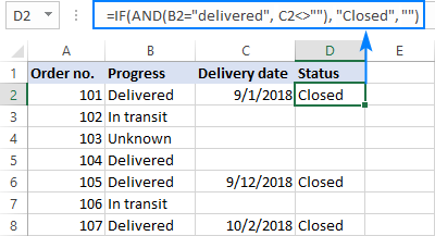
As an example, let's make a formula that checks if B2 is "delivered" and C2 is not empty, and depending on the results, does one of the following:
- If both conditions are TRUE, mark the order as "Closed".
- If either condition is FALSE or both are FALSE, then return an empty string ("").
=IF(AND(B2="delivered", C2<>""), "Closed", "")
The screenshot below shows the IF AND function in Excel:
If you'd like to return some value in case the logical test evaluates to FALSE, supply that value in the value_if_false argument. For example:
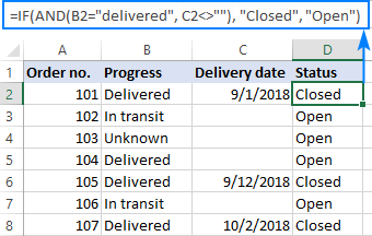
=IF(AND(B2="delivered", C2<>""), "Closed", "Open")
The modified formula outputs "Closed" if column B is "delivered" and C has any date in it (non-blank). In all other cases, it returns "Open":
Note. When using an IF AND formula in Excel to evaluate text conditions, please keep in mind that lowercase and uppercase are treated as the same character. If you are looking for a case-sensitive IF AND formula, wrap one or more arguments of AND into the EXACT function as it is done in the linked example.
Now that you know the syntax of the Excel IF AND statement, let me show you what kind of tasks it can solve.
Excel IF: greater than AND less than
In the previous example, we were testing two conditions in two different cells. But sometimes you may need to run two or more tests on the same cell. A typical example is checking if a cell value is between two numbers. The Excel IF AND function can easily do that too!
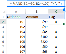
Let's say you have some sales numbers in column B and you are requested to flag the amounts greater than $50 but less than $100. To have it done, insert this formula in C2 and then copy it down the column:
=IF(AND(B2>50, B2<100), "x", "")

If you need to include the boundary values (50 and 100), use the less than or equal to operator (<=) and greater than or equal to (>=) operator:
=IF(AND(B2>=50, B2<=100), "x", "")
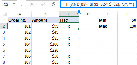
To process some other boundary values without changing the formula, enter the minimum and maximum numbers in two separate cells and refer to those cells in your formula. For the formula to work correctly in all the rows, be sure to use absolute references for the boundary cells ($F$1 and $F$2 in our case):
=IF(AND(B2>=$F$1, B2<=$F$2), "x", "")
By using a similar formula, you can check if a date falls within a specified range.
For example, let's flag dates between 10-Sep-2018 and 30-Sep-2018, inclusive. A small hurdle is that dates cannot be supplied to the logical tests directly. For Excel to understand the dates, they should be enclosed in the DATEVALUE function, like this:
=IF(AND(B2>=DATEVALUE("9/10/2018"), B2<=DATEVALUE("9/30/2018")), "x", "")
Or simply input the From and To dates in two cells ($F$1 and $F$2 in this example) and "pull" them from those cells by using the already familiar IF AND formula:
=IF(AND(B2>=$F$1, B2<=$F$2), "x", "")

For more information, please see Excel IF statement between two numbers or dates.
IF this AND that, then calculate something
Apart from returning predefined values, the Excel IF AND function can also perform different calculations depending on whether the specified conditions are TRUE or FALSE.
To demonstrate the approach, we will be calculating a bonus of 5% for "Closed" sales with the amount greater than or equal to $100.
Assuming the amount is in column B and the order status in column C, the formula goes as follows:
=IF(AND(B2>=100, C2="closed"), B2*10%, 0)

The above formula assigns zero to the rest of the orders (value_if_false = 0). If you are willing to give a small stimulating bonus, say 3%, to orders that do not meet the conditions, include the corresponding equation in the value_if_false argument:
=IF(AND(B2>=100, C2="closed"), B2*10%, B2*3%)

Multiple IF AND statements in Excel
As you may have noticed, we have evaluated only two criteria in all the above examples. But there is nothing that would prevent you from including three and more tests in your IF AND formulas as long as they comply with these general limitations of Excel:
- In Excel 2007 and higher, up to 255 arguments can be used in a formula, with a total formula length not exceeding 8,192 characters.
- In Excel 2003 and lower, no more than 30 arguments are allowed, with a total length not exceeding 1,024 characters.
As an example of multiple AND conditions, please consider these ones:
- Amount (B2) should be greater than or equal to $100
- Order status (C2) is "Closed"
- Delivery date (D2) is within the current month
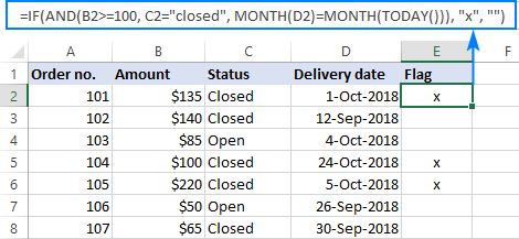
Now, we need an IF AND statement to identify the orders for which all 3 conditions are TRUE. And here it is:
=IF(AND(B2>=100, C2="Closed", MONTH(D2)=MONTH(TODAY())), "x", "")
Given that the 'current month' at the moment of writing was October, the formula delivers the below results:
Nested IF AND statements
When working with large worksheets, chances are that you may be required to check a few sets of different AND criteria at a time. For this, you take a classic Excel nested IF formula and extend its logical tests with AND statements, like this:
To get the general idea, please look at the following example.
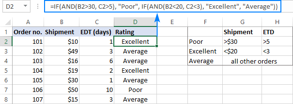
Supposing you want to rate your service based on the shipment cost and estimated time of delivery (ETD):
- Excellent: shipment cost under $20 and ETD under 3 days
- Poor: shipment cost over $30 and ETD over 5 days
- Average: anything in between
To get it done, you write two individual IF AND statements:
IF(AND(B2<20, C2<3), "Excellent", …)
IF(AND(B2>30, C2>5), "Poor", …)
…and nest one into the other:
=IF(AND(B2>30, C2>5), "Poor", IF(AND(B2<20, C2<3), "Excellent", "Average"))
The result will look similar to this:
More formula examples can be found in Excel nested IF AND statements.
Case-sensitive IF AND function in Excel
As mentioned in the beginning of this tutorial, Excel IF AND formulas do not distinguish between uppercase and lowercase characters because the AND function is case-insensitive by nature.
If you are working with case-sensitive data and want to evaluate AND conditions taking into account the text case, do each individual logical test inside the EXACT function and nest those functions into your AND statement:
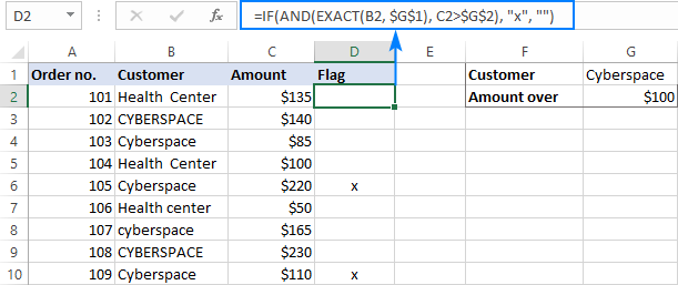
For this example, we are going to flag orders of a specific customer (e.g. the company named Cyberspace) with an amount exceeding a certain number, say $100.
As you can see in the below screenshot, some company names in column B look the same excerpt the characters case, and nevertheless they are different companies, so we have to check the names exactly. The amounts in column C are numbers, and we run a regular "greater than" test for them:
=IF(AND(EXACT(B2, "Cyberspace"), C2>100), "x", "")
To make the formula more flexible, you can input the target customer name and amount in two separate cells and refer to those cells. Just remember to lock the cell references with $ sign ($G$1 and $G$2 in our case) so they won't change when you copy the formula to other rows:
=IF(AND(EXACT(B2, $G$1), C2>$G$2), "x", "")
Now, you can type any name and amount in the referenced cells, and the formula will flag the corresponding orders in your table:
IF OR AND formula in Excel
In Excel IF formulas, you are not limited to using only one logical function. To check various combinations of multiple conditions, you are free to combine the IF, AND, OR and other functions to run the required logical tests. Here is an example of IF AND OR formula that tests a couple of OR conditions within AND. And now, I will show you how you can do two or more AND tests within the OR function.
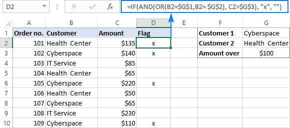
Supposing, you wish to mark the orders of two customers with an amount greater than a certain number, say $100.
In the Excel language, our conditions are expressed in this way:
OR(AND(Customer1, Amount>100), AND(Customer2, Amount>100)
Assuming the customer names are in column B, amounts in column C, the 2 target names are in G1 and G2, and the target amount is in G3, you use this formula to mark the corresponding orders with "x":
=IF(OR(AND(B2=$G$1, C2>$G$3), AND(B2=$G$2, C2>$G$3)), "x", "")
The same results can be achieved with a more compact syntax:
=IF(AND(OR(B2=$G$1,B2= $G$2), C2>$G$3), "x", "")
Not sure you totally understand the formula's logic? More information can be found in Excel IF with multiple AND/OR conditions.
That's how you use the IF and AND functions together in Excel. Thank you for reading and see you next week!
Practice workbook
IF AND Excel – formula examples (.xlsx file)
 by
by
458 comments
I am looking for a formula that does the following for an answer in cell J2:
If cell B2=300 then =SUM(D2)*0.03
If cell B2=400 then =SUM(D2)*0.04
If cell B2=500 then =SUM(D2)*0.05
In other words, cell J2 will calculate IF cell B2 is equal to 300, 400 or 500...then the result will calculate the amount in cell D2 and multiply it by 0.03,0.04 or 0.05.
I thought this was simple enough...but can't quite get it right. Any assistance would be greatly appreciated!
Hello!
You can use this formula:
=IF(B2=300,D2*0.03,IF(B2=400,D2*0.04,IF(B2=500,D2*0.05,"")))
or
=IFS(B2=300,D2*0.03,B2=400,D2*0.04,B2=500,D2*0.05)
You can learn more about multiple conditions and nested IF in Excel in this article.
The formula SUM(D2) doesn't make sense.
Please help me
This is the formula i am using
IF(AND(E6>0,F6>0,I6="PS"), "Yes", IF(AND(F6>0,I6="OP"), "Yes", "No"))
Cell value are E6=1, F6=0, I6=PS, I6= OP
In evaluating formula from Formulas>Evaluate Formula showing #N/A but the output is correct.
IF(False,#N/A, IF(AND(F6>0,I6="OP"), "Yes", "No"))
How to over come #N/A
Hi!
I have not been able to replicate your problem. Perhaps a formula is written in cell F6. When checking the condition F6> 0 using Evaluate Formula, Excel tries to calculate it and gets an error. Evaluate Formula cannot evaluate the formula in another cell.
Date USD GBP AUD
01-04-21 72 105 55
18-04-21 72.5 104.5 55.25
02-05-21 71 102 53.8
15-05-21 72.4 103 55
01-06-21 73.25 105 56
Date Amount Ex.Rate Total
02-04-21 USD 10.25 PLEASE SUGGEST FORMULA TO GET APPlICABLE EXCANGE RATE AS PER THE DATE AND CURRENCY SYMBOL
01-04-21 GBP 10.40
01-04-21 AUD 25.50
05-04-21 USD 220.10
03-04-21 GBP 105.80
04-04-21 AUD 205.25
01-04-21 USD 150.50
02-04-21 GBP 150.18
18-05-21 USD 165.25
10-05-21 AUD 190.75
30-05-21 USD 135.25
Help!
• Shipping Cost which is the cost based on the Region and weight
How do I get this using the two tables below?
i tried If (and but it is very long and I'm getting confused any suggestions?
A B C D E
1 Region Weight Shipping Cost
2 North America 1
3 Asia 0.5
4 Caribbean 5
5 Caribbean 2
6 Caribbean 7.9
7 North America 20
8 Shipping Origination 0.5 – 5 Kg 5.1 – 10 kg 10.1 – 15 kg Over 15 kg
9 South America $5,000 $8,000 $12,000 $15,000
10 Europe $18,000 $10,000 $15,000 $18,000
11 Caribbean $2,000 $6,000 $13,000 $18,000
12 Africa $20,000 $25,000 $35,000 $50,000
13 Australia $25,000 $35,000 $47,000 $60,000
14 Asia $20,000 $31,000 $45,000 $58,000
15 North America $3,000 $6,500 $13,350 $18,770
Region Weight QTY Cost
North America 1 3 $1,230.00
Asia 0.5 21 $3,330.00
Caribbean 5 3 $3,340.00
Caribbean 2 54 $3,350.00
Caribbean 7.9 21 $2,330.00
North America 20 32 $54,310.00
HOW CAN WE CALL LOWER VALUE AGAINST SOME FILED LIKE THAT
CONTAINER VALUE
ABCS1234567 1
ABCS1234567 2
ABCS1234567 3
ABCS1234567 4
WE NEED LOWER VALUE AGAINST SAME CONTAINER NUMBER
IN EXL
THANKS
Hi!
Based on your description, it is hard to completely understand your task. However, I’ll try to guess and offer you the following formula:
=MIN(FILTER(B1:B10,$A$1:$A$10=A1))
HOW CAN WE CALL LOWER VALUE AGAINST SOME FILED LIKE THAT
CONTAINER VALUE
ABCS1234567
you can try this
=IF(AND(L13>0,L134,L138,L1316,L1320,L1342,L1350,"25")))))))
Hi there,
Did I get a situation with 6 conditions, How to write this excel formula?
OD Allowance
O≤Ø4 0.8mm
Ø4<O≤Ø8 1.5mm
Ø8<O≤Ø16 2.0mm
Ø16<O≤Ø20 2.5mm
Ø20<O≤Ø42 3.5mm
O≤Ø50 5mm
The allowance must add to the Actual OD value。 In other words, Actual OD + Allowance, actual OD varies ranging 0 to 50 and above.
Hope to hear from you.
Thank you.
Hello!
A similar problem is solved in this comment.
I am looking for help with a formula.
Column C is the Application Date
Column D is the Application Expiration Date. Formula in that cell is: =IF(C132="","No Start Date",DATE(YEAR(C132)+3,MONTH(C132),DAY(C132)))
Column E is "Days Left". That formula, and I don't know if it's correct or not is: =IF(D133="No Start Date","0",D133-TODAY())
Column F is where I need help. Base Date off of a Today Date of 5/20/2021
Column C Column D Column E Column F
App Date Exp Date Days Left STATUS
2/08/2011 11/10/2020 -191
No Start Date 0
3/11/2019 3/11/2022 295
5/29/2018 5/29/2021 9
What I want is a formula that would be in the STATUS Column that states IF Column E is 0 or less as in a negative number, I want the STATUS to read "EXPIRED. If the Days Left number is =1, I want it to read "RENEW NOW" AND if possible, if Column D Reads "No Start Date", I want the STATUS to read "No Start Date"
Thanks for your help. I have not been able to get any formula to work.
Hello!
If I got you right, the formula below will help you with your task:
=IFS(E132<=0,"Expired", E132=1,"RENEW NOW", C132="","No Start Date",E132>1,"")
or
=IF(E132<=0,"Expired", IF(E132=1,"RENEW NOW", IF(C132="","No Start Date",IF(E132>1,""))))
Here is the article that may be helpful to you: Nested IF in Excel – formula with multiple conditions.
You can learn more about IFS function in Excel in this article on our blog.
Hi,
I am trying to use a toggle to say, if the cell = 1, answer is cell a, if the cell = 2, answer is cell b, if the cell = 3, answer is cell c etc. How would I solve this?
Hello!
I recommend using the CHOOSE function in this case. You can use a nested IF function, but the formula will be more complex.
I hope I answered your question. If something is still unclear, please feel free to ask.
I have been using two different formulas to get my data but I would like to combine them.
Example: Cell (D) has a date (30 June 2021)
Cell (E) might have a date or might not have one : (blank)
In Cell (I) I want to subtract Cell (d) and cell (E). But if Cell (E) does not have a date use "DATE"
Two formulas are:
=IF(ISBLANK(D8),"",-DATE(2021,4,1)+D8) used if there is no date in cell (E)
=IF(E8="","NA",$D8-E8) Used if there is a date in Cell (E)
How would I combine these?
Thank you,
Delila
Hi,
Based on your description, it is hard to completely understand your task. However, I’ll try to guess and offer you the following formula:
=IF(E8="",IF(ISBLANK(D8),"",-DATE(2021,4,1)+D8),$D8-E8)
Trying to create a conditioning format with a number that looks like this ($20.00). I need all numbers greater then that in a range of ($20.00) to ($500.00) to be highlight white letters and back fill, but it will not do it? I know it is something so simple I am hitting wrong?
Hello!
Please check out the following article on our blog, it’ll be sure to help you with your task: Change background color in Excel based on cell value.
select entire cell value and then go to conditional formatting > Select Between > then Chang value what you want for range and then Custom format then change font and background color whatever you want.
Formula on Sheet A =IF(AND('Sheet B'!$A:$A=$C165,'Sheet B'!$D:$D="6",'Sheet B'!$L:$L less than greater than symbol "Completed"),'Sheet B'!$P:$P,0)
not sure why the sign will not show between $L:$L and "Completed", but is in my formula on my sheet.
Need help with this:
Customer Name - Sheet A Column C = Customer ABC (a list of 166 Customers)
Customer Name - Sheet B Column A = Customer ABC (a list of 166 Customers)
Customer Folder - Sheet B Column D = Folder #6 (folders range from 1-6)
Customer Completed - Sheet B Column L = Blank, Not Started, WIP or Completed
Days to Complete - Sheet B Column P = from today to ETA (this can also be a negative if it is pass due)
Want to know in a particular folder how many days to complete if not completed.
Formula on Sheet A =IF(AND('Sheet B'!$A:$A=$C165,'Sheet B'!$D:$D="6",'Sheet B'!$L:$L"Completed"),'Sheet B'!$P:$P,0)
Results have = 0 regardless of the true results.
Correction:
Formula on Sheet A =IF(AND('Sheet B'!$A:$A=$C165,'Sheet B'!$D:$D="6",'Sheet B'!$L:$L"Completed"),'Sheet B'!$P:$P,0)
Hello!
Unfortunately, without seeing your data it is difficult to give you any advice. I'm sorry, it is not very clear what result you want to get. Could you please describe your task in more detail and send us a small sample workbook with the source data and expected result to support@ablebits.com? Please shorten your tables to 10-20 rows/columns and include the link to your blog comment.
We'll look into your task and try to help.
Requirement Shortfall
stock month 1 month 2 month 3 month 1 month 2 month 3
item A 300 400 500 600 -100 -500 -600
item B 100 50 400 600 0 -350 -600
item C 200 50 100 100 0 0 -50
how to calculate shortfall for three months
Hi,
If I understood correctly, you need to use the SUM function
I hope it’ll be helpful.
Thanks for this, But I can't seem to manage my formula.
I need to know the following:
If value (D1) is 5000 and 10000 and 20000 then 4
=IF(D15000,2,IF(D1=10000, 3,IF(D1=20000,4)))))
Afterwards I need to know how many times there was 1,2,3 and 4 in the formula row of course.
What am I doing wrong?
Thanks in advance!
Hello!
To count the number of values, use the COUNTIF function, for example:
=COUNTIF(D1:D100,1)
You can learn more about COUNTIF function in Excel in this article on our blog.
Hi Alexander,
thanks for your reply.
can I share my Excel file with you?
Hi,
thanks for sharing such amazing excel stuff.
I will be grateful if you can help me with this formula:
=IF(AND($F$3=1,M6>L6),J6*M6,J6*L6,IF(AND($F$3=2,N6>M6),J6*N6,J6*M6,IF(AND($F$3=3,O6>N6),J6*O6,J6*N6,IF(AND($F$3=4,P6>O6),J6*P6,J6*O6,IF(AND($F$3=5,Q6>P6),J6*Q6,J6*P6)))))
I am trying to calculate value of work done for each month , (F3 is custome list of months from 1 to 12)
M6 is Jan 21 and L6 is Dec 20 and J6 contract value. if the subsquent month is zero or less than previous month % than, the value should arrive from previous month % multiplied by contract Value.
Kind regards,
Hussain
Hi,
The information you provided is not enough to understand your case and give you any advice, sorry. But I see J6*M6. Are you multiplying the date by a number? Also, your IF functions are not nested within each other, but simply written one after the other.
Here is the article that may be helpful to you: Nested IF in Excel – formula with multiple conditions.
Please describe your problem in more detail. Include an example of the source data and the result you want to get. It’ll help me understand your request better and find a solution for you.
=IF(AND(Z14>89%,AF5=0),"LOW RISK"),IF(AND(Z14>59%,Z140,AF54,"HIGH RISK")
Hello, community.
I have been straggling to right a formula based on the below parameters, is there anyone here that can give a hand, it will be highly appreciated.
- Low Risk = 90% to 100%
- Medium Risk = 60% to 89%
- High Risk = 59% and below
Critical risks: Critical risks are raised when scores an "NC" on any items deemed "critical risk" in the checklist.
Note1: If 3 or less critical risks are raised, the overall risk level shall be at least "Medium" or "High" if the score is below 59%.
Note2: If 4 or more critical risks are raised, the risk level shall be "High" regardless of the score.
I wrote it, in this way but still don't get the logic right.
Being:
Z14 =the cells that contain the score in percentage
AF5= number of high-risk questions scored.
=IF(AND(Z14>89%,AF5=0),"LOW RISK"),IF(AND(Z14>59%,Z140,AF54,"HIGH RISK")
Hi,
Based on your description, it is hard to completely understand your task. However, I’ll try to guess and offer you the following formula:
=IF(AF5 > = 4,"High",IF(Z14 < 59%,"High",IF(Z14 < 89%,"Medium","Low")))
I hope this will help
Hello
I'm not experienced with excel at all and I am try to create a formula on a number of conditions.
It is
IF B="X" and E="Y" then the value at F = D/1.1
but also
If B="x" but E is not "Y" then the value at F = D
but also
If B is not "x" then the value at F =0
Thank you for your assistance as it is doing my head in.
Gary
Hello!
I hope you have studied the recommendations in the tutorial above. It contains answers to your question.
=IF(AND(B1="X",E1="Y"),D1/1.1, IF(AND(B1="X",E1<>"Y"),D1,IF(B1<>"X",0,"")))
I hope I answered your question.
Hello Alexander,
Thank you for your assistance. Formula works perfectly and I have been able to adapt it to other calculations.
Gary
Hello
Good Afternoon!
I'm Here From UAE i just want to ask some questions regarding IFS function.
Please see below Problems.
Thanks in advance.
Cell A2 Where i will Input the data then Cell A3 will be the Output when i Input the data from A2 other data will appear in Cell A3 as an output.
While using the formula in IFS Function the formula is not working in other text value like this "4000-323-1-5"
Formula: A3 Cell =IFS($D$2=4000-323-1-5,"SCS",$D$2=2,"CCTV",$D$2=3,"GBS",$D$2=4,"IPTV",$D$2=5,"IPTEL",$D$2=6,"DNS",$D$2=7,"HSIA",$D$2=8,"PA-BGM",$D$2=9,"GRMS",$D$2=10,"ACS-BOH / GR ACS",TRUE,"")
When i input the data in Cell A2 = 4000-323-1-5 the data that will appear in Cell A3 as an Output is Empty.
But when i input the data in Cell A2 = 2 , 3 , 4 , 5 , 6 , 7 , 8 , 9 and 10 Data is appearing in Cell A3 as per the Formula showing.
Please help me to find what error is coming when i Type the data at Cell A2 as 4000-323-1-5 the data output in Cell A3 is empty. Or please give me a solution how to fix it.
Hello
Please find the revised Message i put it in a wrong cell as per in the formula.
Good Afternoon!
I'm Here From UAE i just want to ask some questions regarding IFS function.
Please see below Problems.
Thanks in advance.
Cell D2 Where i will Input the data then Cell D3 will be the Output when i Input the data from D2 other data will appear in Cell D3 as an output.
While using the formula in IFS Function the formula is not working in other text value like this "4000-323-1-5"
Formula: D3 Cell =IFS($D$2=4000-323-1-5,"SCS",$D$2=2,"CCTV",$D$2=3,"GBS",$D$2=4,"IPTV",$D$2=5,"IPTEL",$D$2=6,"DNS",$D$2=7,"HSIA",$D$2=8,"PA-BGM",$D$2=9,"GRMS",$D$2=10,"ACS-BOH / GR ACS",TRUE,"")
When i input the data in Cell D2 = 4000-323-1-5 the data that will appear in Cell D3 as an Output is Empty.
But when i input the data in Cell D2 = 2 , 3 , 4 , 5 , 6 , 7 , 8 , 9 and 10 Data is appearing in Cell D3 as per the Formula showing that is Equal to 2 = cctv , 3 = gbs.
Please help me to find what error is coming when i Type the data at Cell D2 as 4000-323-1-5 the data output in Cell D3 is empty. Or please give me a solution how to fix it.
Hello!
4000-323-1-5 is a text that consists of numbers. Therefore, in your formula, it must be enclosed in quotes.
=IFS($D$2="4000-323-1-5", ”SCS”,$D$2=2,”CCTV”,$D$2=3,”GBS”,$D$2=4,”IPTV”,$D$2=5, ”IPTEL”,$D$2=6,”DNS”,$D$2=7,”HSIA”,$D$2=8,”PA-BGM”,$D$2=9, ”GRMS”,$D$2=10,”ACS-BOH / GR ACS”,TRUE,””)
I cannot check the work of your formula, since it contains unique links to your data.
I hope my advice will help you solve your task.
Hi!
Good Afternoon!
Dear Mr. Alexander,
Thanks for the Support now the formula is working you are right i just need to put this strings ("").
The best article teaching you how to use IF AND OR formula in Excel!!
Trying to write if statement that analyzes a number within in single cell and returns 1 of the following 3 options:
-- if number in cell is greater than or equal to 10, then take the date in another cell and add 3,650 days
OR
-- if number in cell is less than 10, but greater than or equal to 5, then take the date in another cell and add 1,4650 days
OR
-- if number in cell is less than 5, then take the date in another cell and add 730 days
I had this formula but it is not picking up the less than 5 group
=IF(H3>=10,G3+3650,IF(H3<10,G3+1460,IF(H3<5,G3+730)))
Can anyone help?
Disregard, I was able it figure it out.
=IF(AND(H2>=10,H2=5,H2=0,H2<5),G2+760,"Error-Recheck")))
Have following data
ABCD
Column A credit days 60,90,75,30,
Column b actual days 143,200,115,28
Column C Deviation -83,-110,-40,2
Column D Deviation % 138%,122%,53%,-7%
Column E required : If column D >100% then column A/2, If D50% then A*3/4, If D<50% then A
First two conditions are working but not the last one. Pl help me in fixing this issue.
Using 365
This going to be pretty elaborate so im doing my best to describe whats going on.
I have two sheets..one is called Summary and the other is called Cost.
The Summary has 4 drop downs, which in A9 drop down I am to choose my paint system. The other three drop downs, D7, D8 and D9 i am to choose my surface preps...i can have one, two or three surface preps, depending on the job.
Paint system choices in A9: I have 39 choices, ...the main one driving a majority of the formula is TSA....so id choose either TSA or one of the other 38 choices (im not going to list them all..to much to list)
Surface Prep choices for D7,D8 and D9 are as follows (they all pull from the same list):
N/A
LPWC
SP2
SP3
SP6
SP7
SP10
SP11
SP15
I can chose any combination of the above surface preps in the three drop downs.
On the cost sheet, L28 ( which is the cell the formula will be in) it should populate the existing values in cells L21 or L25, based on the 4 drop down selections on the Summary.
The criteria for L28 populating would be as follows:
If A9 on Summary equals TSA and D7,D8 and D9 contain any one or more of the following in any combination: SP3, SP6, SP7, SP10, SP11, SP15 then give me the value in L25.
So for an example, I can have this as a combo:
A9=TSA
D7=SP10
D8=SP11
D9=SP2
If I have that above combo then I should have the value of L25 show up in L28. There may be a scenario where D8 and D9 will have the choice of N/A...(that means for this particular job only one surface prep was required, not three, but i still have to make a choice in D8 and D9 so I made N/A a choice and in this case I would still get the value of L25 because SP10 and SP11 is in the combination of the three.)
On to the next criteria:
If A9 on Summary equals anything but TSA and D7,D8 and D9 contain any one or more of the following in any combination: SP3, SP6, SP7, SP10, SP11, SP15 then give me the value in L21.
For example, to get the value of L21 to show up in L28, I would have this combo:
A9= anything but TSA (I have 39 choices in this drop down...so im chosing any one of the other 38 options)
D7=LPWC
D8=SP2
D9=SP3
In that scenario above im choosing anything but TSA in A9 ..and again, if D7,D8 and D9 contain any one or more of the following, in any combination: SP3, SP6, SP7, SP10, SP11, SP15 then this time give me the value in L21....(N/A could be a choice too but since I have that SP3 in there, then L21 value should still show up in L28)
The combo to leave L28 at zero would be anything but TSA in A9 and any one or more of the following combinations in D7, D8 and D9: SP2 , LPWC
A9 = anything but TSA
D7=LPWC
D8=SP2
D9=N/A
So basically the only time L28 is left at zero is if anything but TSA is in A9 and the only surface prep is SP2 and/or LPWC.
That pretty much sums up what im looking for. I hope I was as precise and clear as possible.
Thanks for your time and reading and possibly helping me out.
here is the formula for my description above:
=IF(Summary!B9="TSA",IF(OR(OR(Summary!D9="SP3",Summary!D9="SP6",Summary!D9="SP7",Summary!D9="SP10",Summary!D9="SP11",Summary!D9="SP15"),OR(Summary!D8="SP3",Summary!D8="SP6",Summary!D8="SP7",Summary!D8="SP10",Summary!D8="SP11",Summary!D8="SP15"),OR(Summary!D7="SP3",Summary!D7="SP6",Summary!D7="SP7",Summary!D7="SP10",Summary!D7="SP11",Summary!D7="SP15")),L25,""),IF(OR(OR(Summary!D9="SP3",Summary!D9="SP6",Summary!D9="SP7",Summary!D9="SP10",Summary!D9="SP11",Summary!D9="SP15"),OR(Summary!D8="SP3",Summary!D8="SP6",Summary!D8="SP7",Summary!D8="SP10",Summary!D8="SP11",Summary!D8="SP15"),OR(Summary!D7="SP3",Summary!D7="SP6",Summary!D7="SP7",Summary!D7="SP10",Summary!D7="SP11",Summary!D7="SP15")),L21,0))
I am trying a conditional statement with this logic:
If Q101ABS(Q101), then Q101*0.01672
If Q101<0 and K101<Q101, then K101*0.01672
If neither statement is true, then return a blank cell.
This is what I tried that doesn't work
=IF(AND(Q101ABS(Q101)),Q101*0.01672),IF(AND(Q101<0,K101<Q101), K101*0.01672,"")
ty for your help.
I am trying to write a formula which will return answers based on data within the 'I' column, plus return a blank cell if column 'D' is blank. I've tried the following two formulas (based on information you provided to another user which I now can't find in the chat thread):
=IF(I2="Retaliation","TO DO","NA",IF(AND(D2=""),"").
The first half of the formula works, but when I add my IF/AND statement it fails.
=IF(AF2="Not determined","NA",IF(AF2="Substantiated","TO DO",IF(AND(G2=""),"")))
The response I get is "FALSE".
I have checked for typos multiple times but clearly I'm missing something. I hope you can provide some guidance!
Hello!
If I understand your task correctly, the following formula should work for you:
=IF(D2="","",IF(I2="Retaliation","TO DO","NA"))
Hope this is what you need.
Trying to build an if and statement If in a column there are multiple Letters but each letter = a word.
Hello!
The information you provided is not enough to understand your case and give you any advice, sorry. Could you please describe it in more detail? What result do you want to get?
I'm sure this is simple but I can not seem to figure out how to get it to work.
Cell M9 is dependent on what happens in cell L9
if L9 is greater than or equal to 3, M9 should be "P",
if L9 is less than 3, M9 should be zero
if L9 is equal to "D", M9 should be zero
if L9 is equal to "N", M9 should be zero
What is the best way to make this happen - if it is possible to make happen?
Thanks
D
Oh.... I got it. Sorry. I knew it was easy, but my mind is fried.
Sorry.
Ok.... but I still have a problem.
So..... the initial part of the formula is obviously =IF(L9>=3,"P")
I have another column that is counting the "P"s, another counting the "D"s, and another counting the "N"s. So here is the problem. When I type in a "D" (for instance) in L9, M9 is putting a "P" in the column and thus, being counted in the "P" count. Also happens if I type a "N" in L9.... a "P" shows up in M9. So I definitely need to know how to make M9 appear as a zero when typing either a "D" or an "N" in L9.
I was think the If/And/or formula would work but can't seem to get the correct combination of things.
So ….. yea, I could still use some help on this.
thanks again
d
=IF(L9="D",0)*AND(L9="N",0)*OR(L9>=3,"P")
This is the formula I was trying. It woks until I add the "OR" part. is it because it two different types of functions? the first two are dealing with alpha characters and the 3rd with a numeric?
I didn't think it would be, but I could be wrong.
Hello!
If I got you right, the formula below would help you with your task:
=IF(OR(L9="D",L9="N"),0,IF(L9>=3,"P",0 ))
Hope this is what you need.
Alexander,
Thank you so much.
I see now why mine didn't work.
I really appreciate the help.
It totally works now!!!!
D
Sorry, even though my formula shows correctly to me, by the time it sends it changes to something else, interesting!
Sorry, when I cut and pasted the formula did not paste correctly:
=IF(B27=7,B27=11,B27=14,B27<=16),4)
Here is the formula I created, but it returns nothing but "0". I am trying to assign a scale of 1-4 for the following brackets:
0-6=1
7-10=2
11-13=3
14-16=4
=IF(B27=7,B27=11,B27=14,B27<=16),4)
Any help is greatly appreciated!
Hello!
I’m sorry but your task is not entirely clear to me. Could you please describe it in more detail? What result do you want to get? Thank you!
if a1>=b1 then a1=5
if a1<b1 then a1=0
How to join above in one formular??
Kindly help
Hello!
A formula cannot refer to the cell in which it is written.
Hi,
I have a pivot table with three invoice types: X,Y,Z paid from two POs: A & B. I need to separate invoice X to be paid out of A, and Y&Z to be paid out of B. How should I write my IF function to add Y&Z to be paid out of B?
Hello!
I’m sorry but your task is not entirely clear to me. For me to be able to help you better, please describe your task in more detail. Please specify what you were trying to find, what formula you used and what problem or error occurred. Give an example of the source data and the expected result.
It’ll help me understand it better and find a solution for you
I'm unsure why the following formula is not working. I tested all 3 separately and they function correctly but not when I put them together. When I use them together the result is always "Not Started", even when I add text to C3 and a date to I3.
=IF(ISTEXT(E3), "Not Started",IF(AND(ISTEXT(E3),ISTEXT(C3)), "In Process", IF(AND(ISTEXT(E3),ISTEXT(C3),ISNUMBER(I3)), "Complete")))
can you add a bit more context to your post. its a little vague as to what you're trying to do.
=IF(AND(D2>55,E2>65),"Passed both Theory and Practical"),IF(AND(D2>55,E2<65),"Passed Theory and Failed Practical Assessment"),IF(AND(D265),"Passed Practical Assessment Failed Theory Assessment"),IF(AND(D2>55,E2>65),"Unsuccessful"))))))
Hi,
Try this:
=IF(AND(D2>=55,E2>=65),"Passed both Theory and Practical",IF(AND(D2<55,E2=55,E2<65),"Passed Theory and Failed Practical Assessment",IF(AND(D2=65),"Passed Practical Assessment Failed Theory Assessment",""))))
I hope that helps :)
OOPS sorry thta one has a typo, the correct one is below:
=IF(AND(D2>=55,E2>=65),"Passed both Theory and Practical",IF(AND(D2<55,E2=55,E2<65),"Passed Theory and Failed Practical Assessment",IF(AND(D2=65),"Passed Practical Assessment Failed Theory Assessment",""))))
Ok for some reason this website is changing my posts:
after this bit:
This part of the formula: IF(AND(D2<55,E2=55,E2=55,E2>=65),"Passed both Theory and Practical", IF(AND(D2<55,E2=55,E2<65),"Passed Theory and Failed Practical Assessment", IF(AND(D2=65),"Passed Practical Assessment Failed Theory Assessment",""))))
jeez this is frustrating me remove the e2=55, bit
IF DEBIT DAYS 0-31 OR SEC.=2,"5%", SEC=1,"4.5%", SEC=0,"3"AND DEBIT DAYS 31-62 OR SEC=2,"4%", SEC=1,"2%",SEC=0,"1.5%" AND UP TO 62 ,"0" HOW PUT IF FORMULA
I'm looking for a formula that will calculate how much someone gets paid if they work 46.50 hours a week with the following criteria (36-37 hours paid at regular pay, 37-45 paid @1.5x, 45 hours and above paid @ 2x). Regurla pay is $25/per hour.
Hello Adam!
The formula below will do the trick for you:
=(MAX(0,C1-45)*2+MIN(MAX(0,C1-37),8)*1.5+MIN(MAX(0,C1-36),1)*1)*25
This can replace the IF and AND functions.
Please may someone help me with a If/And formula?
I'm working on a formula to highlight if annual spend is 50% higher than estimated spend.BUT ignore if estimated spend value is blank.
I have a simple - If A1(spend) is greater than B1(estimted spend), yes or no. (Below)
=IF(A1>B1,"Yes","No")
But i'm struggling to understand how i can expand that to ignore if B1 value is blank?
Any help would be greatly appreciated - thank you.
Hello Catherine!
If I understand your task correctly, the following formula should work for you:
=IF(A1<>"",IF(A1>B1,"Yes","No"),"")
I hope this will help
I am looking to combine the following 2 statements:
=IF((AND(D3="Put",F3>E3)), ((E3-F3)*(B3*C3)), 0)
=IF((AND(D3="Call",F3<E3)), ((F3-E3)*(B3*C3)), 0)
They work independently from one another but I cannot figure out how to combine them. The goal is to use the correct formula depending on what I have in D3 (Call or Put).
Some guidance would be greatly appreciated.
Thanks.
I've worked it out on my own.
Hello Rob!
If I got you right, the formula below will help you with your task:
=IF(D3="Put",IF(F3 > E3,((E3-F3)*(B3*C3)),0), IF((AND(D3="Call",F3 < E3)), ((F3-E3)*(B3*C3)), 0))
This will combine the two IF formulas
hello sir,
i want count sunday of till date in excel
=COUNTIFS(L9:AO9,"sun")it give me 4 sunday, whole month of june-2020(date 01/06/2020 to 30/06/2020)
i want for till date like =countifs(01/06/2020:10/06/2020,"sun")
How can I do this with excel formula?
if possible please suggest or help me
jai
Hello!
I recommend that you read the COUNTIFS Feature Guide. Please describe your problem in more detail. Include an example of the source data and the result you want to get. It’ll help me understand your request better and find a solution for you. Thank you.
Set 1 Set 2 Set 3 Result
Y N N AA
N N Y BB
Y N Y CC
N Y N DD
Y Y N EE
Y Y Y FF
N Y Y GG
N N N HH
Need help with the logic formula - Conditions to be used are only IF, AND. OR.
Hi Shariff,
Is the formula below what you're looking for?
=if(and(A1="Y",B1="N",C1="N"),"AA",if(and(A1="N",B1="N",C1="Y"),"BB",if(and(A1="Y",B1="N",C1="Y"),"CC",if(and(A1="N",B1="Y",C1="N"),"DD",if(and(A1="Y",B1="Y",C1="N"),"EE",if(and(A1="Y",B1="Y",C1="Y"),"FF",if(and(A1="N",B1="Y",C1="Y"),"GG",if(and(A1="N",B1="N",C1="N"),"HH",""))))))))
ASD DFG SDF Result
Y N N AA
N N Y BB
Y N Y CC
N Y N DD
Y Y N EE
Y Y Y FF
N Y Y GG
N N N HH
Need help with the logic formula - Conditions to be used are only IF, AND. OR.
Hello!
I’m sorry but your task is not entirely clear to me. Could you please describe it in more detail? Thank you!
I have two cells that are binary either 1 or 0 so I have 4 variables
A1=0, A2=0
A1=0, A2=1
A1=1, A2=0
A1=1, A2=1
and I need a cell to determine what the cells are and if of example
A1=0, A2=0 then cell A3= open
A1=0, A2=1 then cell A3= Right
A1=1, A2=0 then cell A3= Left
A1=1, A2=1 then cell A3= Short
How can I do this with excel formula?
Thanks
Eddie
Hello Eddie!
If I understand your task correctly, the following formula should work for you:
=IF(AND(A1=0,A2=0),"Open", IF(AND(A1=0,A2=1),"Right", IF(AND(A1=1,A2=0),"Left", IF(AND(A1=1,A2=1),"Short",""))))
I hope it’ll be helpful.
HI, I have 2 tables, one table has information on Base quantity, another table has the following information;
Sales/ M for Jan & Feb Average Monthly Base starting at Growth of average of Jan&Feb
> 15000 10%
> 10000 5%
> 7500 15%
> 5000 20%
how do i simplify the formula in excel
Hello Pankaj!
I’m sorry but your task is not entirely clear to me.
For me to be able to help you better, please describe your task in more detail. Please let me know in more detail what you were trying to find, what formula you used and what problem or error occurred. It’ll help me understand it better and find a solution for you. Thank you.
I have a spreadsheet with over 5000 rows of a machine id all with varying installation dates ranging from 2012 to today. Column A is machine id. Column B is Installed date. In Column C each machine has a classification code about 8 different classes eg Ste, Alu etc. In column D a disposal date. In Column E i have costs for year 2012. Column F for 2013 and so on. If disposed of for eg in 2012 there will be no costs for other yrs. I need to summarise by month by year the count of installations by classification. Then sum by month and year and by classification the costs. What is the best approach and formulas
Any help appreciated
Hello Lizzy!
The easiest and most correct way to get an answer to your questions is to use a pivot table. Our blog has many articles about this. I recommend here and here.
I hope it’ll be helpful.
Easy to follow explanation