This tutorial explains the difference between the SUMIF and SUMIFS functions in terms of their syntax and usage, and provides a number of formula examples to sum values with multiple AND / OR criteria in Excel 365, 2021, 2019, 2016, 2013, 2010, and lower.
As everyone knows, Microsoft Excel provides an array of functions to perform various calculations with data. A few articles ago, we explored COUNTIF and COUNTIFS, which are designed for counting cells based on a single condition and several conditions, respectively. Last week we covered Excel SUMIF that adds values meeting the specified criteria. Now it's time to go over the plural version of SUMIF - Excel SUMIFS that allows summing values by multiple criteria.
Those who are familiar with the SUMIF function might think that converting it to SUMIFS takes just an extra "S" and a few additional criteria. This would seem quite logical… but "logical" it's not always the case when dealing with Microsoft : )
Excel SUMIF function - syntax & usage
The SUMIF function is used to conditionally sum values based on a single criteria. We discussed the SUMIF syntax in detail in the previous article, and here's just a quick refresher.
- range - the range of cells to be evaluated by your criteria, required.
- criteria - the condition that must be met, required.
- sum_range - the cells to sum if the condition is met, optional.
As you see, the syntax of the Excel SUMIF function allows for one condition only. And still, we say that Excel SUMIF can be used to sum values with multiple criteria. How can that be? By adding the results of several SUMIF functions and by using SUMIF formulas with array criteria, as demonstrated in the examples that follow.
Excel SUMIFS function - syntax & usage
You use SUMIFS in Excel to find a conditional sum of values based on multiple criteria. The SUMIFS function was introduced in Excel 2007 and is available in all subsequent versions of Excel 2010, 2013, 2016, 2019, 2021, and Excel 365.
Compared to SUMIF, the SUMIFS syntax is a little bit more complex:
The first 3 arguments are mandatory, additional ranges and their associated criteria are optional.
sum_range- one or more cells to sum, required. This can be a single cell, a range of cells or a named range. Only cells with numbers are summed; blank and text values are ignored.criteria_range1- the first range to be evaluated by the associated criteria, required.criteria1- the first condition that must be met, required. You can supply the criteria in the form of a number, logical expression, cell reference, text or another Excel function. For example you can use criteria such as 10, ">=10", A1, "cherries" or TODAY().criteria_range2, criteria2, …- these are additional ranges and criteria associated with them, optional. You can use up to 127 range/criteria pairs in SUMIFS formulas.
Notes:
- For a SUMIFS formula to work correctly, all the criteria_range arguments must have the same dimension as sum_range, i.e. the same number of rows and columns.
- The SUMIFS function works with AND logic, meaning that a cell in the sum range is summed only if it meets all of the specified criteria, i.e. all the criteria are true for that cell.
Basic SUMIFS formula
And now, let's have a look at the Excel SUMIFS formula with two conditions. Suppose, you have a table listing the consignments of fruit from different suppliers. You have the fruit names in column A, suppliers' names in column B, and quantity in column C. What you want is to find out a sum of amounts relating to a given fruit and supplier, e.g. all apples supplied by Pete.
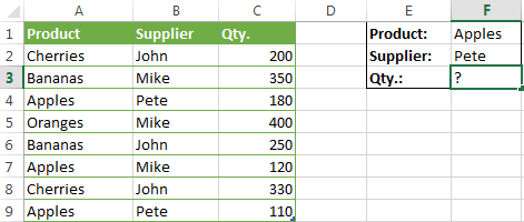
When you're learning something new, it's always a good idea to start with simple things. So, to begin with, let's define all the arguments for our SUMIFS formula:
- sum_range - C2:C9
- criteria_range1 - A2:A9
- criteria1 - "apples"
- criteria_range2 - B2:B9
- criteria2 - "Pete"
Now assemble the above parameters, and you will get the following SUMIFS formula:
=SUMIFS(C2:C9, A2:A9, "apples", B2:B9, "Pete")
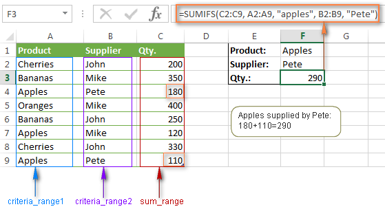
To refine the formula further, you can replace the text criteria "apples" and "Pete" with cell references. In this case, you won't have to change the formula to calculate the quantity of other fruit from a different supplier:
=SUMIFS(C2:C9, A2:A9, F1, B2:B9, F2)
Note. Both the SUMIF and SUMIFS functions are case-insensitive by nature. To get them to recognize the text case, please see Case-sensitive SUMIF and SUMIFS formula in Excel.
SUMIF vs. SUMIFS in Excel
Since the aim of this tutorial is to cover all possible ways to sum values by several conditions, we will discuss formula examples with both functions - Excel SUMIFS and SUMIF with multiple criteria. To use them correctly, you need to clearly understand what these two functions have in common and in what way they are different.
While the common part is clear (similar purpose and parameters), the differences are not so obvious, though very essential.
There are 4 major differences between SUMIF and SUMIFS:
- Number of conditions. SUMIF can evaluate just one condition at a time while SUMIFS can check for multiple criteria.
- Syntax. With SUMIF, the sum_range is the last and optional argument - if not defined, the values in the range argument are summed. With SUMIFS, sum_range is the first and required argument.
- Size of ranges. In SUMIF formulas, sum_range does not necessarily have to be of the same size and shape as range, as long as you have the top left cell right. In Excel SUMIFS, each criteria_range must contain the same number of rows and columns as the sum_range argument.
For example, SUMIF(A2:A9,F1,C2:C18) will return the correct result because the leftmost cell in the sum_range argument (C2) is right. So, Excel will make the correction automatically and include as many columns and rows in sum_range as there are in range.
A SUMIFS formula with unequally sized ranges will return a #VALUE! error.
- Availability. SUMIF is available in all Excel versions, from 365 through 2000. SUMIFS is available in Excel 2007 and higher.
Alright, enough strategy (i.e. theory), let's get into the tactics (i.e. formula examples : )
How to use SUMIFS in Excel - formula examples
A moment ago, we discussed a simple SUMIFS formula with two text criteria. In the same manner, you can use Excel SUMIFS with multiple criteria expressed by numbers, dates, logical expressions, and other Excel functions.
Example 1. Excel SUMIFS with comparison operators
In our fruit suppliers table, suppose, you want to sum all deliveries by Mike with Qty. 200 or more. To do this, you use the comparison operator "greater than or equal to" (>=) in criteria2 and get the following SUMIFS formula:
=SUMIFS(C2:C9,B2:B9,"Mike",C2:C9,">=200")
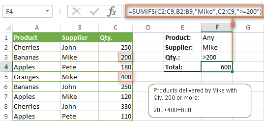
Note. Please pay attention that in Excel SUMIFS formulas, logical expressions with comparison operators should always be enclosed in double quotes ("").
We covered all possible comparison operators in detail when discussing Excel SUMIF function, the same operators can be used in SUMIFS criteria. For example, the following formula with return the sum of all values in cells C2:C9 that are greater than or equal to 200 and less than or equal to 300.
=SUMIFS(C2:C9, C2:C9,">=200", C2:C9,"<=300")
Example 2. Using Excel SUMIFS with dates
In case you want to sum values with multiple criteria based on the current date, use the TODAY() function in your SUMIFS criteria, as demonstrated below. The following formula sums values in column D if a corresponding date in column C falls within the last 7 days, including today:
=SUMIFS(D2:D10, C2:C10,">="&TODAY()-7, C2:C10,"<="&TODAY())
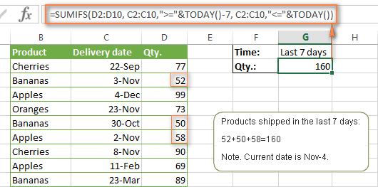
Note. When you use another Excel function together with a logical operator in the criteria, you have to use the ampersand (&) to concatenate a string, for example "<="&TODAY().
In a similar fashion, you can use the Excel SUMIF function to sum values in a given date range. For example, the following SUMIFS formula adds the values in cells C2:C9 if a date in column B falls between 1-Oct-2014 and 31-Oct-2014, inclusive.
=SUMIFS(C2:C9, B2:B9, ">=10/1/2014", B2:B9, "<=10/31/2014")
The same result can be achieved by calculating the difference of two SUMIF functions, as demonstrated in this example - How to use SUMIF to sum values in a given date range. However, Excel SUMIFS is much easier and more understandable, isn't it?
Example 3. Excel SUMIFS with blank and non-blank cells
When analyzing reports and other data, you may often need to sum values corresponding either to empty or non-empty cells.
| Criteria | Description | Formula Example | |
|---|---|---|---|
| Blank cells | "=" | Sum values corresponding to blank cells that contain absolutely nothing - no formula, no zero length string. | =SUMIFS(C2:C10, A2:A10, "=", B2:B10, "=")
Sum values in cells C2:C10 if the corresponding cells in columns A and B are absolutely empty. |
| "" | Sum values corresponding to "visually" blank cells including those that contain empty strings returned by some other Excel function (for example, cells with a formula like =""). | =SUMIFS(C2:C10, A2:A10, "", B2:B10, "")
Sum values in cells C2:C10 with the same conditions as the above formula, but includes empty strings. |
|
| Non-blank cells | "<>" | Sum values corresponding to non-empty cells, including zero length strings. | =SUMIFS(C2:C10, A2:A10, "<>", B2:B10, "<>")
Sum values in cells C2:C10 if the corresponding cells in columns A and B are not empty, including cells with empty strings. |
| SUM-SUMIF or SUM / LEN |
Sum values corresponding to non-empty cells, not including zero length strings. | =SUM(C2:C10) - SUMIFS(C2:C10, A2:A10, "", B2:B10, "")
=SUM((C2:C10) * (LEN(A2:A10)>0)*(LEN(B2:B10)>0)) Sum values in cells C2:C10 if the corresponding cells in columns A and B are not empty, cells with zero length strings are not included. |
And now, let's see how you can use a SUMIFS formula with "blank" and "non-blank" criteria on real data.
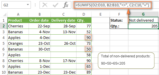
Suppose, you have an order date in column B, delivery date in column C and Qty. in column D. How do you find the total of products that have not been delivered yet? That is, you want to know the sum of values corresponding to non-empty cells in column B and empty cells in column C.
The solution is to use the SUMIFS formula with 2 criteria:
=SUMIFS(D2:D10, B2:B10,"<>", C2:C10,"=")
Using Excel SUMIF with multiple OR criteria
As noted in the beginning of this tutorial, the SUMIFS function is designed with AND logic. But what if you need to sum values with multiple OR criteria, i.e. when at least one of the conditions is met?
Example 1. SUMIF + SUMIF
The simplest solution is to sum the results returned by several SUMIF functions. For example, the following formula demonstrates how to find the total of products delivered by Mike and John:
=SUMIF(C2:C9,"Mike",D2:D9) + SUMIF(C2:C9,"John",D2:D9)
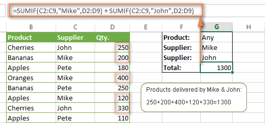
As you see, the first SUMIF function adds the quantities corresponding to "Mike", the other SUMIF function returns the amounts relating to "John" and then you add these 2 numbers.
Example 2. SUM & SUMIF with an array argument
The above solution is very simple and may get the job done quickly when there are only a couple of criteria. But a SUMIF + SUMIF formula may grow up enormously if you want to sum values with multiple OR conditions. In this case, a better approach is using an array criteria argument in the SUMIF function. Let's examine this approach now.
You can start by listing all of your conditions separated by commas and then enclose the resulting comma-separated list in {curly brackets}, which is technically called an array.
In the previous example, if you want to sum the products delivered by John, Mike and Pete, your array criteria will look like {"John","Mike","Pete"}. And the complete SUMIF function is SUMIF(C2:C9, {"John","Mike","Pete"} ,D2:D9).
The array argument consisting of 3 values forces your SUMIF formula to return three separate results, but since we write the formula in a single cell, it would return the first result only - i.e. the total of products delivered by John. To get this array-criteria approach to work, you have to use one more little trick - enclose your SUMIF formula in a SUM function, like this:
=SUM(SUMIF(C2:C9, {"John","Mike","Pete"} , D2:D9))
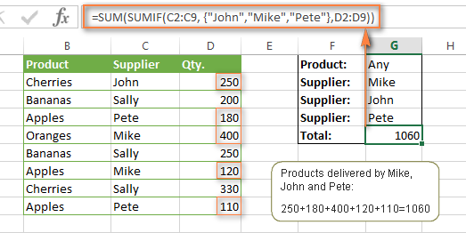
As you see, an array criteria makes the formula much more compact compared to SUMIF + SUMIF, and lets you add as many values as you like in the array.
This approach works with numbers as well as with text values. For instance, if instead of the suppliers' names in column C, you had supplier IDs like 1, 2, 3 etc., then your SUMIF formula would look similar to this:
=SUM(SUMIF(C2:C9, {1,2,3} , D2:D9))
Unlike text values, numbers needn't be enclosed in double quotes in array arguments.
Example 3. SUMPRODUCT & SUMIF
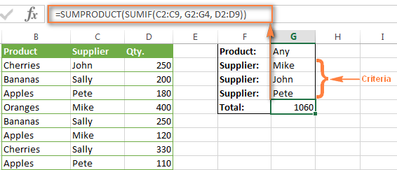
In case, your preferred way is to list the criteria in some cells rather that specify them directly in the formula, you can use SUMIF in conjunction with the SUMPRODUCT function that multiplies components in the given arrays, and returns the sum of those products.
=SUMPRODUCT(SUMIF(C2:C9, G2:G4, D2:D9))
Where G2:G4 are the cells containing your criteria, the suppliers' names in our case, as illustrated in the screenshot below.
But of course, nothing prevents you from listing the values in an array criteria of your SUMIF function if you want to:
=SUMPRODUCT(SUMIF(C2:C9, {"Mike","John","Pete"}, D2:D9))
The result returned by both formulas will be identical to what you see in the screenshot:
Excel SUMIFS with multiple OR criteria
If you want to conditionally sum values in Excel not simply with multiple OR conditions, but with several sets of conditions, you will have to use SUMIFS instead of SUMIF. The formulas will be very similar to what we've just discussed.
As usual, an example might help to illustrate the point better. In our table of fruit suppliers, let's add the Delivery Date (column E) and find the total quantity delivered by Mike, John and Pete in October.
Example 1. SUMIFS + SUMIFS
The formula produced by this approach includes a lot of repetition and looks cumbersome, but it is easy to understand and, most importantly, it works : )
=SUMIFS(D2:D9,C2:C9, "Mike", E2:E9,">=10/1/2014", E2:E9, "<=10/31/2014") +

SUMIFS(D2:D9, C2:C9, "John", E2:E9, ">=10/1/2014", E2:E9, "<=10/31/2014") +

SUMIFS(D2:D9, C2:C9, "Pete", E2:E9, ">=10/1/2014" ,E2:E9, "<=10/31/2014")
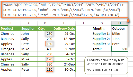
As you see, you write a separate SUMIFS function for each of the suppliers and include two conditions - equal to or greater than Oct-1 (">=10/1/2014",) and less than or equal to Oct 31 ("<=10/31/2014"), and then you sum the results.
Example 2. SUM & SUMIFS with an array argument
I've tried to explain the essence of this approach in the SUMIF example, so now we can simply copy that formula, change the order of arguments (as you remember it is different in SUMIF and SUMIFS) and add additional criteria. The resulting formula is more compact than SUMIFS + SUMIFS:
=SUM(SUMIFS(D2:D9,C2:C9, {"Mike", "John", "Pete"}, E2:E9,">=10/1/2014", E2:E9, "<=10/31/2014"))
The result returned by this formula is exactly the same as you see in the screenshot above.
Example 3. SUMPRODUCT & SUMIFS
As you remember, the SUMPRODUCT approach differs from the previous two in the way that you enter each of your criteria in a separate cell rather that specify them directly in the formula. In case of several criteria sets, the SUMPRODUCT function won't suffice and you will have to employ ISNUMBER and MATCH as well.
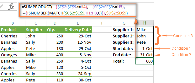
So, assuming that the Supplies Names are in cells H1:H3, Start Date is in cell H4 and End Date in cell H5, our SUMPRODUCT formula takes the following shape:
=SUMPRODUCT(--(E2:E9>=H4), --(E2:E9<=H5), --(ISNUMBER(MATCH(C2:C9, H1:H3,0))), D2:D9)
Many people wonder why use double dash (--) in SUMPRODUCT formulas. The point is that Excel SUMPRODUCT ignores all but numeric values, while the comparison operators in our formula return Boolean values (TRUE / FALSE), which are non-numeric. To convert these Boolean values to 1's and 0's, you use the double minus sign, which is technically called the double unary operator. The first unary coerces TRUE/FALSE to -1/0, respectively. The second unary negates the values, i.e. reverses the sign, turning them into +1 and 0, which the SUMPRODUCT function can understand.
I hope the above explanation makes sense. And even if it doesn't, just remember this rule of thumb - use the double unary operator (--) when you are using comparison operators in your SUMPRODUCT formulas.
Using Excel SUM in array formulas
As you remember, Microsoft implemented the SUMIFS function in Excel 2007. If someone still uses Excel 2003, 2000 or earlier, you will have to use a SUM array formula to add values with multiple AND criteria. Naturally, this approach works in modern versions of Excel 2013 - 2007 too, and can be deemed an old-fashioned counterpart of the SUMIFS function.
In the SUMIF formulas discussed above, you have already used array arguments, but an array formula is something different.
Example 1. Sum with multiple AND criteria in Excel 2003 and earlier
Let's get back to the very first example where we found out a sum of amounts relating to a given fruit and supplier:

As you already know, this task is easily accomplished using an ordinary SUMIFS formula:
=SUMIFS(C2:C9, A2:A9, "apples", B2:B9, "Pete")
And now, let's see how the same task can be fulfilled in early "SUMIFS-free" versions of Excel. First off, you write down all the conditions that should be met in the form of range="condition". In this example, we have two range/condition pairs:
Condition 1: A2:A9="apples"
Condition 2: B2:B9="Pete"
Then, you write a SUM formulas that "multiplies" all of your range/condition pairs, each enclosed in brackets. The last multiplier is the sum range, C2:C9 in our case:
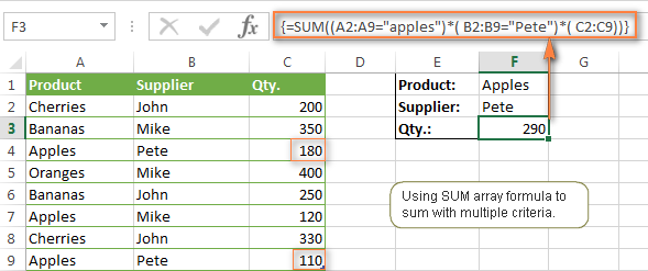
=SUM((A2:A9="apples") * ( B2:B9="Pete") * ( C2:C9))
As illustrated in the screenshot below, the formula perfectly works in the latest Excel 2013 version.
Note. When entering any array formula, you must press Ctrl + Shift + Enter. Once you do this, your formula gets enclosed in {curly braces}, which is a visual indication that an array formula is entered correctly. If you try typing the braces manually, your formula will be converted to a text string, and it won't work.
Example 2. SUM array formulas in modern Excel versions
Even in modern versions of Excel, the power of the SUM function should not be underestimated. The SUM array formula is not simply gymnastics of the mind, but has a practical value, as demonstrated in the following example.
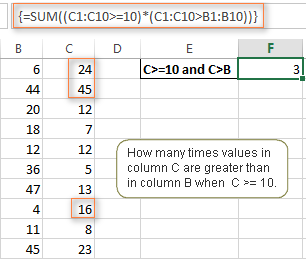
Suppose, you have two columns, B and C, and you need to count how many times column C is greater than column B, when a value in column C is greater or equal to 10. An immediate solution that comes to mind is using the SUM array formula:
=SUM((C1:C10>=10) * (C1:C10>B1:B10))
Don't see any practical application to the above formula? Think about it in another way : )
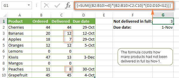
Suppose, you have the orders list like shown in the screenshot below and you want to know how many products have not been delivered in full by a given date. Translated into Excel's language, we have the following conditions:
Condition 1: A value in column B (Ordered items) is greater than 0
Condition 2: A value in column C (Delivered) in less than in column B
Condition 3: A date in column D (Due date) is less than 11/1/2014.
Putting the three range/condition pairs together, you get the following formula:
=SUM((B2:B10>=0)*(B2:B10>C2:C10)*(D2:D10<G2))
Well, the formula examples discussed in this tutorial have only scratched the surface of what Excel SUMIFS and SUMIF functions can really do. But hopefully, they have helped pointing you in the right direction and now you can sum values in your Excel workbooks no matter how many intricate conditions you have to consider.
 by
by
666 comments
Awesome and fantastic concepts by the owner who imparted basic and advance concepts lots of thanks !!!!!!!!!!
invoice num doc date amount
20000056 24.01.2017 536
20000057 23.01.2017 765
20000058 24.01.2017 897
20000059 23.01.2017 545
20000060 24.01.2017 7654
20000061 23.01.2017 897
20000062 24.01.2017 987
20000063 23.01.2017 651
20000064 12.12.2016 210
20000065 01.10.2016 610
20000066 01.10.2016 211
20000067 23.01.2016 109
20000068 23.01.2017 187
94000011 23.01.2016 145
94000012 23.01.2017 167
94000013 23.01.2016 198
94000014 23.01.2016 103
94000017 23.01.2016 1765
94000019 23.01.2016 543
94000032 23.01.2016 532
94000033 23.01.2016 346
94000034 23.01.2016 678
I juat want to know that which all invoices I should add to get exact 3000
I am having trouble coming up with a proper formula for this:
This is a list of positions open and when it was filled.
Site Status Created Filled
A FT 1/1/2000 1/2/2000
B FT 1/2/2000 2/1/2000
C P 1/3/2000
A P 1/4/2000
B FT 1/5/2000 2/1/2000
C P 1/6/2000
A FT 1/7/2000 1/4/2000
B P 1/8/2000
C P 1/9/2000
I am trying to write a formula that basically asks, If site = x, then sum 8 for FT and 6 for PT, for each entry if my date in question falls between the created and filled dates. Also if the filled date is blank that means it's still open. So that needs to be included.
My gut tells me it should be an index/match formula (or vlookup) which i've done in the past.
This is the forumla that i have so far =SUMIFS(Hours,Site, "="&B3, Status, "="&D3, Created, ""&C3)
I created a new column that listed the status as a number.
Name Amount 1099 Y/N
A (250) N
A (2,546.58) Y
B 184.50 N
C (3,500.00) Y
B (1,500.00) N
Hi, if I want to sum if 1099 column indicates "Y" by "Name" so that it will populate A with "Y" ...B with "Y" ..so forth. how do i formulate the functions?
I'm trying to avoid sumifs + sumifs + ...
I have multiple criteria in my data table (date, location, type, subtype) that must match. I'd like to be able to have location and type look to a list for criteria rather than hard code, as I need to use similar function 15 or more times and prefer to change the list reference than typing in and hard-coding the names, places as they change.
sumifs(C:C,B:B,list1,A:A,datecell,D:D,sitelist)
Above is oversimplified as I reference 4-5 criteria ranges
it works when I reference 1 list and it seems that either I have a bad list reference of it won't allow criteria to be lists in 2 places.
can you help?
Appreciate your help with the below formula..
Col A Col B
>=10M 10
=10M 30
using the below formula
=SUMIFS(B2:B4,A2:A4,">=10M")
I am getting result 0 but expecting 40...Using Sumifs as there are other criteria as well along with the above formule..
Thanks in advance..
I see some data is missing..
so to add on to above ">=10M" is a static value not an operator..
Hi,
Is it possible to get the value of a specific cell as your criteria1 or criteria2 ? ex. =SUMIFS(T8:T109,R8:R109,"value inside cell AE6",S8:S109,"value inside cell AE7")
thank you very much for your response. :)
thanks
Dear
Greetings..!
I'm trying to calculate SUMIF function but i do not know how to calculate and getting my answer but i would expecting you guys will solve my problem in excel.
i have an excel sheet that contain in Column (A) Date as (1-1-2016 1:00 PM) in Column (B) Names Like (Adam, John, Wiki) in Column (C) an Amount such as 100, 200, 500 in Column (D) Should be My Answer that's are follows
if in Column (A) Date "1-1-2016 to 31-1-2016" and in Column (B) "Adam" then Calculate the amount in Column (C) "100" and show the Addition in Column (D)
i tried this but i'm fail
=SUMIFS(C1:C3,B1:B3,"Adam")+SUMIFS(C1:C3,B1:B3,">=1-01-2016",A1:A3,"<=31-01-2016")
Kindly Help me
Thanks in Advance
=SUM(SUMIFS(C2:C18,B2:B18,"Del",A2:A18,">=1-Jan-17",A2:A18,"<=15-Jan-17"))
Question regarding Cells Contain non empty "alone".....
Sum Values in Cells C2:C10, if the Corresponding cells in Columns A2,A5,A6,A10's are filled in with totals, remaining A3,A4,A7,A9's are filled in with values. Now I want Sum only Filled in with totals and not values and next condition is totals <10000 should come. I tried below formula but all values are coming(A2,A3,A4,A5,A6,A7,A8,A9,A10).
=SUMIFS(C2:C10,A2:A10,"",C2:C10,"<10000")
Please give me some solution for the above, Thanking You
Hi, thanks for your great article, this helped a lot!
Can you please help me to split an array out of the formula into a different cell to make it easier to update?
=SUMPRODUCT(SUMIF('data'!$B:$B,{"Apples","Oranges","Pears"},'data'!$J:$J))
In the above formula, I wish to change it to something like =SUMPRODUCT(SUMIF('data'!$B:$B,C3,'data'!$J:$J)), where C3 contains {"Apples","Oranges","Pears"}.
Is this possible?
Thanks!
In columns A, B & C I have a list of names. All the names are the same for each column just not each column will have a complete list of all the names nor will it be in order. (See below). My question is this: I need a formula in column D that will tell me
1) if a name in column C matches a name in columns A and B to say "good"
2) if the name in column C matches a name in column A but not B to say "scanned"
3) if the name in column C matches a name in column B but not in column A to say "timesheet".
Example:
A B C D
Adriana Alvin Alvin GOOD
Alvin Tony N/A N/A
Anthony Adriana Anthony SCANNED
Sam Sam Tony TIMESHEET
HI,
USING IF CONDITION HOW WE CAN ADD VALUES LIKE
A1 APPLE 03PCS
A2 ORANGE 8PCS
A3 BANANA 2PCS
A4 APPLE 13PCS
A5 APPLE 07PCS
A6 ORANGE 10PCS
A7 BANANA 4PCS
IF I NEED TO CALCULATE ONLY THE QUANTITY OF AN APPLE USING IF CONDITION WHAT WOULD BE THE FORMULA
Hello, I'm a beginner and a teacher who really needs help with creating my formula. I want the formula to report the number in column 1 if the numbers in the column is between 1 - 4 but add column 1 to 2 if column 1 is 5 or more. If column 1 and 2 is greater than 10, I want it to add column 3 otherwise just say the sum of 1 and 2. This goes on for quite some time and so the function often breaks or doesn't work properly. Any tips on how to do this? I tried to write a formula with the if function but it didn't work well. I'd be grateful for any and every tip. Thanks, T.
Hi!
If my understanding of the task is correct, the following formula should work a treat:
=IF(A2<5, A2, IF(A2+B2>10, A2+B2+C2, A2+B2))
please see attached
Hi Gabriel
=IFERROR((Z19/AD19),0)
or
=IF(AA19=0,0,Z19/AA19)
I would do the first one personally. Hope it helps!
Michel, I would just add another column with =IF(G2<100,SUM(G2*250)*H2,H2*G2)
I was hoping someone might give me some insight into how I can combine these two functions:
=SUM(Z19/AD19)
=IF(AD19,Z19/AD19,0)
The SUM is delivering a #DIV/0!
This leads to the IF statement which delivers a "0" so it can be read by some conditional formatting I have listed.
I need the cell to be able to read the SUM and calculate when it can (and it does) but if the division is by "0" and I get the #DIV/0! I need that IF calculation to produce the "0"
Can anyone help please?
Gabriel
Hi
I want to include a SUMIF in a SUMPROUCT formula where a value should change if it is lower than a specific value.
=SUMPRODUCT((G2:G36,H2:H36)/SUMIF(G2:G36,"<100", G2:G36*250))
The above function does not work, however, if value(number) in the "G" row is lower than 100, it should be multiplied by 250.
I cannot get it to work...hope you can help.
Thanks
Hi i have a List of number that i wanted to know which of the SUM(combination) that will match with my predefine value.
Example:
In column A1 i have this list of number
100,110,130,150,160
and i wanted to know which of the summation will get 260
i want to sum non-blanks in a row of data after bypassing first three non-blanks. Means I have to sum from the start of 4th non-blank entries without considering first three non-blanks. please support.
Hello,
please I need to fix formula for:
I have to make 3 flights within 90 days.
in C/D/E I have dates of each flight. I have to know if 3 flights are done within 90 days. and according to last date-3rd date ( if 3 flights are done in 90 days)I have to know expiry date, means + 90
thanks
I have an excel file where I capture the estimated working hours of the employee from the website in Sheet1(employee working hours), I need to capture the estimated and actual hours, whichever has the higher hours will be shown in the cell in sheet2(Utilization sheet).
=SUMIFS('From employee working hours'!P:P,'From employee working hours'!Y:Y,'Utilization sheet'!D5,'From employee working hours'!K:K,'Utilization sheet!$C$1, 'From Dashboard'!U:U,"")
- it shows the estimated working hours, the actual hours is from From employee working hours'!Q:Q
hi How can i convert 10010101 into Aplha-numeric A-01-01-01 where digit at first two places 10=A
please show me how to calculate 8 in a cell + RDO in another cell to equel 16
Hello, need help. I want to calculate the amount payable to driver "A" for the pickups and/or deliveries done between 19:00hrs & 01:00 hour on 08/24/16. In this example he should get $10.
No Pdate Ptime Ddate Dtime Amt$
A 8/24/2016 2:10 8/24/2016 5:40 2.00
A 8/24/2016 5:45 8/24/2016 7:40 3.00
A 8/24/2016 17:58 8/24/2016 19:39 5.00
A 8/24/2016 20:30 8/24/2016 22:01 3.00
A 8/24/2016 23:50 8/25/2016 1:05 2.00
No PickupDt PickupTime Delivery Date Delivery Time Drv($)
A 8/24/2016 2:108/24/2016 5:40 2.00
A 8/24/2016 5:45 8/24/2016 7:40 3.00
A 8/24/2016 17:58 8/24/2016 19:39 5.00
A 8/24/2016 20:30 8/24/2016 22:01 3.00
A 8/24/2016 23:50 8/25/2016 1:05 2.00
I need to calculate the amount payable to person A for date 8/22/16 the pickup time and/or delivery time between 19:00hrs & 01:00hrs
No Pickup Date Pickup Time Delivery Date Delivery Time Drv($)
A8/24/2016 2:10 8/24/2016 5:40 2.00
A 8/24/2016 5:45 8/24/2016 7:40 3.00
A 8/24/2016 17:58 8/24/2016 19:39 5.00
A 8/24/2016 20:30 8/24/2016 22:01 3.00
A 8/24/2016 23:50 8/25/2016 1:05 2.00
give some sumif and countifs sumifs,countifs,avg
avgifs problematic examples
Hi,
Can you plz tell me how to solve below mentioned issue.
=SUMIFS(B23:R23,B26:R26,"PAID",B20:R20,"=1/1/2016")
When I put this formula it is working, but what I want is,to change the month of the date when I drag it to other cells in the same raw. It means, the month has to be changed automatically, January 2016, February 2016, March 2016.
=SUMIFS(B23:R23,B26:R26,"PAID",B20:R20,"=1/1/2016")
=SUMIFS(B23:R23,B26:R26,"PAID",B20:R20,"=1/2/2016")
=SUMIFS(B23:R23,B26:R26,"PAID",B20:R20,"=1/3/2016") like this.
How can I get changed only month automatically in this formula. Because all the time I have to change the month of the date manually. Please assist
Dear Admin User,
Please help me, my problem is mentioned the bellow.
1
1202 Need 12000 =sumifs(a6:a10,">5000",b6:b10,"=1",c6:c10,a4)
5000 1 1203
6000 2 1202
6000 2 1202
5000 1 1203
5000 2 1203
5000 2 1202
5000 1 1202
Thanks,
I want to take a single criteria from one column, take a multiple criteria from another column and then sum the final column if the criteria from the first two are there. I know in your world this is a absolutely simple but I'm struggling. I'm looking for PFV in column C,if we have a PFV in column C then we also need 1,2,5,6,45,46,49 or 50 in column E, I then need the sum of the relevant figures in column F. I have to do this for over 100 separate tabs! Thanks for any help you can give me!
In my column A I've all the first name and column B is the last name. When I try to do a sumifs to add any names in Column A it won't give me any result. However, when I do the same sumifs for column B it give me the correct result. How come they can't search the names in Column A. Please advise. Thanks
Hi Frank,
Sorry, it's not possible to determine the source of the problem without seeing the original data. Try typing some names manually in a new sheet, and then try your formula. If it works, then the problem is with the names in the original worksheet, and if it doesn't, then double check the formula.
#DIV/0!
=AVERAGEIFS(Yarn!O$2:O$10000,Yarn!B$2:B$10000,Sheet7!C$1,Yarn!I$2:I$10000,Sheet7!A$3:A$135,Yarn!J$2:J$10000,Sheet7!B$3:B$135)
help me please
Hello Dear All,
I Use Excel 2007, i want to make
E8:E107= Product (Desktop), G8:G107=Technician (Milon), T8:T107=Total Product Value.
i Need to Show Only milon how mutch Keep from Desktop
Suppliers amount
Peter 128089
Peter 128090
Peter 128091
Peter 128092
Peter 128093
Peter 128094
Peter 128095
Peter 128096
Peter 128097
Peter 128098
Peter 128099
Peter 128100
Peter 128101
John 21654114
John 21654115
John 21654116
John 21654117
John 21654118
John 21654119
John 21654120
John 21654121
John 21654122
John 21654123
John 21654124
John 21654125
John 21654126
John 21654127
John 21654128
John 21654129
John 21654130
Tom 48418
Tom 48418
Tom 48418
Tom 48418
Tom 48418
Tom 48418
Tom 48418
Tom 48418
Tom 48418
Tom 48418
Tom 48418
Can you help me for preparing summary sheet?
there're more than 15 suppliers so I wanted to prepare a summary that all of them come just in one sheet.
How to prepare Monthly Payroll in Excel Sheet ?
help me please now and today if possible.
"i have to award DIVISION I, II, III, IV and 0 to my students who have scored different grades in their subjects either A, B, C, D and F where each carries different POINTS such as A=1, B=2,C=3, D=4 and F=5.And note that the minimum subject to be taken by a student is 7 and the maximum is 10 while others can take 8 or 9 is allowed. As well as award division is equivalent to the following points; for Div I =(1-7)points, Div II = (8-12)points, Div III = (13-24)points, Div IV = (25-33)points, Div 0 = (34-35)points. Note that the awarded Division to any students regards/considers to the first seven subject scored highest others less than 7 subjects awarded as INC - incomplete. Thus core subjects are 7 among the taken ones. plz help which formula or function am to apply to award for my class students now.
thanks and be blessed abundantly by God. Amen.
How do I get the total of all Fruit NOT sold by Mike?
Hi Sheil,
You can use a SUMIF formula similar to this:
=SUMIF(B2:B10, "<>"&"mike", C2:C10)
Where B is the column containing the names and C is the column to sum.
Hi, I am trying to calculate a formula for the following data.
t1 t2 t3 TOTAL
-----------------------------
10 10* 10* 20
Critria:
-In this I'm interested in sum of only * marks
like in this total of 3 tests is 20 because there two stars of 10 marks.
Can anyone please guide me?
It is Amazing.
I Love it
Hi, I am trying to calculate a formula for the following data.
Name Gender Grade
---- ------ -----
ABC Male A+
DEF Male A
ACD Female A+
ASD Male A
SDF Female B
AED Male A+
LKJ Male A
LOK Female B
I would like to calculate Following things.
1) Count of Male Students whose Grade is A+?
2) Count of FeMale Students whose Grade is A?
I couldn't able to write the excel formula to find the above things.
Can anyone guide me?
Hello,
I am trying to come up with a formula that populates a sum of numbers from a different sheet (data source) - The tricky part is, I need the formula to cover a few different scenarios.
Here are the things i need to cover:
1. I need all of the items in a certain status (located in one column) that have a date range between 6/3/2016 - 6/9/2016 (located in another column)
2. I need all of the items in 3 different status' (located in the same column) that have a date range between 6/3/2016 - 6/9/2016 (located in another column).
The table I am trying to fill is on a different worksheet within the same workbook. I am having difficulty determining what formula set(s) to use to accomplish this. I will need to repeat the process weekly to have a running total - The data source will also be updated weekly, so these numbers need to be active, not static.
Example:
I need the total of all measures (items) that are in status "1-Template", status "2-Configuration", status "2.1-Reconfig" that were completed between 6/3 - 6/9 - I need this number to be populated into a table I created on sheet 2.
Next, I need all of the measures (items) that are in status "6.3-Production" that were completed between 6/3 - 6/9- I need this number to be populated into a table I created on sheet 2.
The range of the columns for status is A2:A5181
The range of date completed is C2:C5181
Any assistance is greatly appreciated! *I doubt anyone will see this immediately, but if possible, I need this today :) )
1 1
4 2
3 1
2 2
11 1
1 2
4 1
3 2
2 1
11 2
1 1
4 2
3 1
2 2
11 1
1 2
4 1
3 2
2 1
11 2
1 1
4 2
3 1
2 2
11 1
1 2
4 1
3 2
2 1
Fist Colum count only 1, 11 number of count and second Colum 1 number of count please h
Hi,
I am trying to calculate a formula that encompasses more that one cell as a criteria(so I don't have to copy the formula 4 times which each cell.
eg I have list of criteria
DASHBORD
A53 England
A54 America
A55 Scotland
A56 Australia
My formula currently is:
=SUMIFS('Master List'!H:H,'Master List'!I:I,"Ticket",'Master List'!BN:BN,Dashboard!A53)
How do I change Dashboard!A53 to include A54, A55 and A56 eg(A54:A56)
We list our jobs on a WIP (work in progress) worksheet. Column E is the total revenue expected on the job. Column K is our actual cost in dollars of the job. Column P is the % of the job completed based on Cost/Revenue. Column U is the amount invoiced to date. Column X needs to tell us, based on the % complete, less previously invoiced amount, what our projected revenue will be. The part I can't seem to get is how do we tell Column X to only calculate up to 100% of Column P?
If costs exceed 100%, it keeps calculating, telling us our projections need to invoice more then what the expected revenue will be. (Obviously we cant charge the customer more just because we didn't control our costs and keep them under 100%. I need it to only calculate up to 100%.
E: Total Revenue for the job(we enter this amt)
K: Job Costs in Dollar Amount (we enter this amt)
P: Calculated % of Work Complete using the formula cost/revenue
U: Amount invoiced to date (a formula calculating previously invoice + current invoicing)
X: should tell us what our projected revenue is but only up to 100% in column P. Should column P go over 100%, we don't want to use the overage.
I have a sheet that shows planned and actual delivered tonnage for a product.
In the A column I have the delivery date, and in the B column, I have the month number ranging from 1 to 12 based on the date in the A column; in the I column, I have the planned tonnage, and in the J column, I have the actual delivered tonnage. The cells in the J column is blank if no delivery have been done yet.
What I am looking for is a way to make a prognosis calculation based on what has actually been delivered so far this month plus the planned tonnage for the deliveries remaining this month.
Right now, I have a hidden column that either shows the corresponding J cell value if it is bigger than 0 and if not, shows the I value. And then does a summation of this hidden column where the B value corresponds to the month number I am calculating.
Is this possible using functions in Excel?
Hi,
Nice thread.
In your example of =SUM(SUMIF(C2:C9, {"John","Mike","Pete"} , D2:D9))
my equivalent would be =SUM(SUMIF(C2:C9, {"2A","2B","2C"} , D2:D9))
while 2 is determined dynamically within the same sheet say it is in cell E1 and then A, B and C have to be concatenated.
I have tried something like below -
=SUM(SUMIF(C2:C9, {"&E1A","&E1B","&E1C"} , D2:D9))
or
=SUM(SUMIF(C2:C9, {"&E1&"A"","&E1"&B"","&E1"&C""} , D2:D9))
Can you please help?
Is it possible to use sumifs to add numbers based on the letter and the date? For example: the sum of all A for 30-Apr (=6)
29-Feb 31-Mar 30-Apr 31-May
A 1 2 3 4
B 1 2 3 4
C 1 2 3 4
A 1 2 3 4
E 1 2 3 4
C 1 2 3 4
G 1 2 3 4
H 1 2 3 4
This is a great article with a bunch of new tricks I do not know about. My question is that when I used the array argument in a SUMIFS function, the results are calculated from only applying the first argument in the list, and ignored the rest. In your example, when I used {1, 2, 3} as the array argument, the SUMIFS function only returns the calculation based on 1, not including 2 or 3. My excel is from Microsoft Office Professional Plus 2013. When I tried to search "array argument" in Excel Help (clicking the "?" on the upper right corner, there was no relevant entry appeared.
Does this array argument a newer feature than Office 2013 or an older feature but eliminated from Office 2013?
Thanks for your help!
If I want to add up the total spent in a budget heading (a drop down list) for a particular month across sheets why is:
=SUMIFS(Sheet2!D2:D11,Sheet2!A2:A11,"Marketing",Sheet2!C2:C11,"Sep") not working when D is amount spent, A is budget heading and C is date
Thank you
Hello. I've tried to use "sumifs" and "sumproduct" functions, but
seems doing something.
Spreedsheet 1: Column A= dates of one month, column B=list of products on each day of a given month, column C=qty;
Spreedsheet 2: Column A=dates of one month, Column B = need to get sum of a particular items from sheet1 column B, of course taking in account date of selling.
Thank you very much in advance.