This tutorial explains the difference between the SUMIF and SUMIFS functions in terms of their syntax and usage, and provides a number of formula examples to sum values with multiple AND / OR criteria in Excel 365, 2021, 2019, 2016, 2013, 2010, and lower.
As everyone knows, Microsoft Excel provides an array of functions to perform various calculations with data. A few articles ago, we explored COUNTIF and COUNTIFS, which are designed for counting cells based on a single condition and several conditions, respectively. Last week we covered Excel SUMIF that adds values meeting the specified criteria. Now it's time to go over the plural version of SUMIF - Excel SUMIFS that allows summing values by multiple criteria.
Those who are familiar with the SUMIF function might think that converting it to SUMIFS takes just an extra "S" and a few additional criteria. This would seem quite logical… but "logical" it's not always the case when dealing with Microsoft : )
Excel SUMIF function - syntax & usage
The SUMIF function is used to conditionally sum values based on a single criteria. We discussed the SUMIF syntax in detail in the previous article, and here's just a quick refresher.
- range - the range of cells to be evaluated by your criteria, required.
- criteria - the condition that must be met, required.
- sum_range - the cells to sum if the condition is met, optional.
As you see, the syntax of the Excel SUMIF function allows for one condition only. And still, we say that Excel SUMIF can be used to sum values with multiple criteria. How can that be? By adding the results of several SUMIF functions and by using SUMIF formulas with array criteria, as demonstrated in the examples that follow.
Excel SUMIFS function - syntax & usage
You use SUMIFS in Excel to find a conditional sum of values based on multiple criteria. The SUMIFS function was introduced in Excel 2007 and is available in all subsequent versions of Excel 2010, 2013, 2016, 2019, 2021, and Excel 365.
Compared to SUMIF, the SUMIFS syntax is a little bit more complex:
The first 3 arguments are mandatory, additional ranges and their associated criteria are optional.
sum_range- one or more cells to sum, required. This can be a single cell, a range of cells or a named range. Only cells with numbers are summed; blank and text values are ignored.criteria_range1- the first range to be evaluated by the associated criteria, required.criteria1- the first condition that must be met, required. You can supply the criteria in the form of a number, logical expression, cell reference, text or another Excel function. For example you can use criteria such as 10, ">=10", A1, "cherries" or TODAY().criteria_range2, criteria2, …- these are additional ranges and criteria associated with them, optional. You can use up to 127 range/criteria pairs in SUMIFS formulas.
Notes:
- For a SUMIFS formula to work correctly, all the criteria_range arguments must have the same dimension as sum_range, i.e. the same number of rows and columns.
- The SUMIFS function works with AND logic, meaning that a cell in the sum range is summed only if it meets all of the specified criteria, i.e. all the criteria are true for that cell.
Basic SUMIFS formula
And now, let's have a look at the Excel SUMIFS formula with two conditions. Suppose, you have a table listing the consignments of fruit from different suppliers. You have the fruit names in column A, suppliers' names in column B, and quantity in column C. What you want is to find out a sum of amounts relating to a given fruit and supplier, e.g. all apples supplied by Pete.
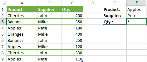
When you're learning something new, it's always a good idea to start with simple things. So, to begin with, let's define all the arguments for our SUMIFS formula:
- sum_range - C2:C9
- criteria_range1 - A2:A9
- criteria1 - "apples"
- criteria_range2 - B2:B9
- criteria2 - "Pete"
Now assemble the above parameters, and you will get the following SUMIFS formula:
=SUMIFS(C2:C9, A2:A9, "apples", B2:B9, "Pete")
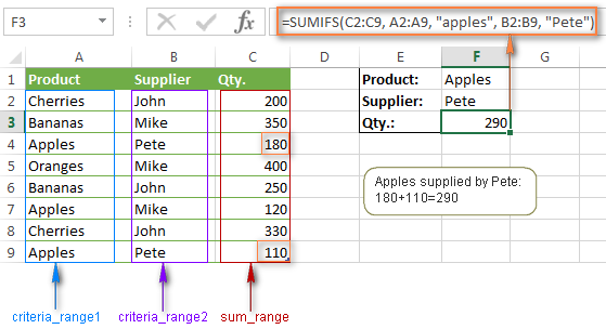
To refine the formula further, you can replace the text criteria "apples" and "Pete" with cell references. In this case, you won't have to change the formula to calculate the quantity of other fruit from a different supplier:
=SUMIFS(C2:C9, A2:A9, F1, B2:B9, F2)
Note. Both the SUMIF and SUMIFS functions are case-insensitive by nature. To get them to recognize the text case, please see Case-sensitive SUMIF and SUMIFS formula in Excel.
SUMIF vs. SUMIFS in Excel
Since the aim of this tutorial is to cover all possible ways to sum values by several conditions, we will discuss formula examples with both functions - Excel SUMIFS and SUMIF with multiple criteria. To use them correctly, you need to clearly understand what these two functions have in common and in what way they are different.
While the common part is clear (similar purpose and parameters), the differences are not so obvious, though very essential.
There are 4 major differences between SUMIF and SUMIFS:
- Number of conditions. SUMIF can evaluate just one condition at a time while SUMIFS can check for multiple criteria.
- Syntax. With SUMIF, the sum_range is the last and optional argument - if not defined, the values in the range argument are summed. With SUMIFS, sum_range is the first and required argument.
- Size of ranges. In SUMIF formulas, sum_range does not necessarily have to be of the same size and shape as range, as long as you have the top left cell right. In Excel SUMIFS, each criteria_range must contain the same number of rows and columns as the sum_range argument.
For example, SUMIF(A2:A9,F1,C2:C18) will return the correct result because the leftmost cell in the sum_range argument (C2) is right. So, Excel will make the correction automatically and include as many columns and rows in sum_range as there are in range.
A SUMIFS formula with unequally sized ranges will return a #VALUE! error.
- Availability. SUMIF is available in all Excel versions, from 365 through 2000. SUMIFS is available in Excel 2007 and higher.
Alright, enough strategy (i.e. theory), let's get into the tactics (i.e. formula examples : )
How to use SUMIFS in Excel - formula examples
A moment ago, we discussed a simple SUMIFS formula with two text criteria. In the same manner, you can use Excel SUMIFS with multiple criteria expressed by numbers, dates, logical expressions, and other Excel functions.
Example 1. Excel SUMIFS with comparison operators
In our fruit suppliers table, suppose, you want to sum all deliveries by Mike with Qty. 200 or more. To do this, you use the comparison operator "greater than or equal to" (>=) in criteria2 and get the following SUMIFS formula:
=SUMIFS(C2:C9,B2:B9,"Mike",C2:C9,">=200")
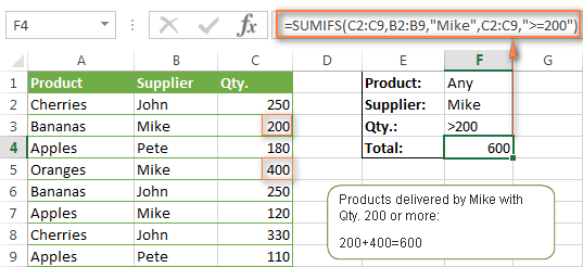
Note. Please pay attention that in Excel SUMIFS formulas, logical expressions with comparison operators should always be enclosed in double quotes ("").
We covered all possible comparison operators in detail when discussing Excel SUMIF function, the same operators can be used in SUMIFS criteria. For example, the following formula with return the sum of all values in cells C2:C9 that are greater than or equal to 200 and less than or equal to 300.
=SUMIFS(C2:C9, C2:C9,">=200", C2:C9,"<=300")
Example 2. Using Excel SUMIFS with dates
In case you want to sum values with multiple criteria based on the current date, use the TODAY() function in your SUMIFS criteria, as demonstrated below. The following formula sums values in column D if a corresponding date in column C falls within the last 7 days, including today:
=SUMIFS(D2:D10, C2:C10,">="&TODAY()-7, C2:C10,"<="&TODAY())
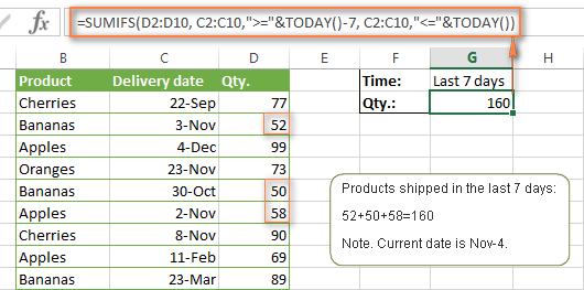
Note. When you use another Excel function together with a logical operator in the criteria, you have to use the ampersand (&) to concatenate a string, for example "<="&TODAY().
In a similar fashion, you can use the Excel SUMIF function to sum values in a given date range. For example, the following SUMIFS formula adds the values in cells C2:C9 if a date in column B falls between 1-Oct-2014 and 31-Oct-2014, inclusive.
=SUMIFS(C2:C9, B2:B9, ">=10/1/2014", B2:B9, "<=10/31/2014")
The same result can be achieved by calculating the difference of two SUMIF functions, as demonstrated in this example - How to use SUMIF to sum values in a given date range. However, Excel SUMIFS is much easier and more understandable, isn't it?
Example 3. Excel SUMIFS with blank and non-blank cells
When analyzing reports and other data, you may often need to sum values corresponding either to empty or non-empty cells.
| Criteria | Description | Formula Example | |
|---|---|---|---|
| Blank cells | "=" | Sum values corresponding to blank cells that contain absolutely nothing - no formula, no zero length string. | =SUMIFS(C2:C10, A2:A10, "=", B2:B10, "=")
Sum values in cells C2:C10 if the corresponding cells in columns A and B are absolutely empty. |
| "" | Sum values corresponding to "visually" blank cells including those that contain empty strings returned by some other Excel function (for example, cells with a formula like =""). | =SUMIFS(C2:C10, A2:A10, "", B2:B10, "")
Sum values in cells C2:C10 with the same conditions as the above formula, but includes empty strings. |
|
| Non-blank cells | "<>" | Sum values corresponding to non-empty cells, including zero length strings. | =SUMIFS(C2:C10, A2:A10, "<>", B2:B10, "<>")
Sum values in cells C2:C10 if the corresponding cells in columns A and B are not empty, including cells with empty strings. |
| SUM-SUMIF or SUM / LEN |
Sum values corresponding to non-empty cells, not including zero length strings. | =SUM(C2:C10) - SUMIFS(C2:C10, A2:A10, "", B2:B10, "")
=SUM((C2:C10) * (LEN(A2:A10)>0)*(LEN(B2:B10)>0)) Sum values in cells C2:C10 if the corresponding cells in columns A and B are not empty, cells with zero length strings are not included. |
And now, let's see how you can use a SUMIFS formula with "blank" and "non-blank" criteria on real data.
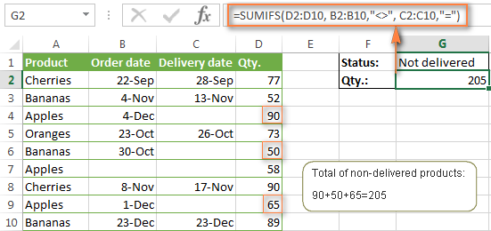
Suppose, you have an order date in column B, delivery date in column C and Qty. in column D. How do you find the total of products that have not been delivered yet? That is, you want to know the sum of values corresponding to non-empty cells in column B and empty cells in column C.
The solution is to use the SUMIFS formula with 2 criteria:
=SUMIFS(D2:D10, B2:B10,"<>", C2:C10,"=")
Using Excel SUMIF with multiple OR criteria
As noted in the beginning of this tutorial, the SUMIFS function is designed with AND logic. But what if you need to sum values with multiple OR criteria, i.e. when at least one of the conditions is met?
Example 1. SUMIF + SUMIF
The simplest solution is to sum the results returned by several SUMIF functions. For example, the following formula demonstrates how to find the total of products delivered by Mike and John:
=SUMIF(C2:C9,"Mike",D2:D9) + SUMIF(C2:C9,"John",D2:D9)
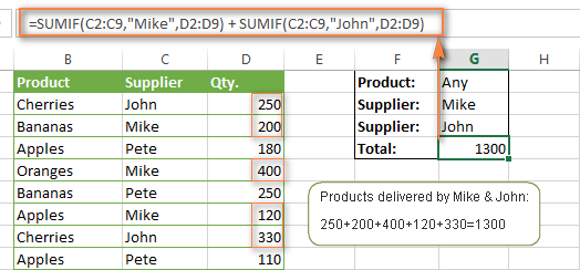
As you see, the first SUMIF function adds the quantities corresponding to "Mike", the other SUMIF function returns the amounts relating to "John" and then you add these 2 numbers.
Example 2. SUM & SUMIF with an array argument
The above solution is very simple and may get the job done quickly when there are only a couple of criteria. But a SUMIF + SUMIF formula may grow up enormously if you want to sum values with multiple OR conditions. In this case, a better approach is using an array criteria argument in the SUMIF function. Let's examine this approach now.
You can start by listing all of your conditions separated by commas and then enclose the resulting comma-separated list in {curly brackets}, which is technically called an array.
In the previous example, if you want to sum the products delivered by John, Mike and Pete, your array criteria will look like {"John","Mike","Pete"}. And the complete SUMIF function is SUMIF(C2:C9, {"John","Mike","Pete"} ,D2:D9).
The array argument consisting of 3 values forces your SUMIF formula to return three separate results, but since we write the formula in a single cell, it would return the first result only - i.e. the total of products delivered by John. To get this array-criteria approach to work, you have to use one more little trick - enclose your SUMIF formula in a SUM function, like this:
=SUM(SUMIF(C2:C9, {"John","Mike","Pete"} , D2:D9))
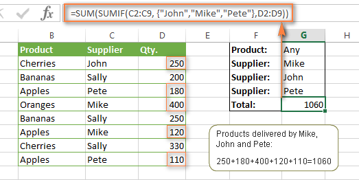
As you see, an array criteria makes the formula much more compact compared to SUMIF + SUMIF, and lets you add as many values as you like in the array.
This approach works with numbers as well as with text values. For instance, if instead of the suppliers' names in column C, you had supplier IDs like 1, 2, 3 etc., then your SUMIF formula would look similar to this:
=SUM(SUMIF(C2:C9, {1,2,3} , D2:D9))
Unlike text values, numbers needn't be enclosed in double quotes in array arguments.
Example 3. SUMPRODUCT & SUMIF
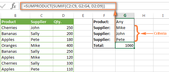
In case, your preferred way is to list the criteria in some cells rather that specify them directly in the formula, you can use SUMIF in conjunction with the SUMPRODUCT function that multiplies components in the given arrays, and returns the sum of those products.
=SUMPRODUCT(SUMIF(C2:C9, G2:G4, D2:D9))
Where G2:G4 are the cells containing your criteria, the suppliers' names in our case, as illustrated in the screenshot below.
But of course, nothing prevents you from listing the values in an array criteria of your SUMIF function if you want to:
=SUMPRODUCT(SUMIF(C2:C9, {"Mike","John","Pete"}, D2:D9))
The result returned by both formulas will be identical to what you see in the screenshot:
Excel SUMIFS with multiple OR criteria
If you want to conditionally sum values in Excel not simply with multiple OR conditions, but with several sets of conditions, you will have to use SUMIFS instead of SUMIF. The formulas will be very similar to what we've just discussed.
As usual, an example might help to illustrate the point better. In our table of fruit suppliers, let's add the Delivery Date (column E) and find the total quantity delivered by Mike, John and Pete in October.
Example 1. SUMIFS + SUMIFS
The formula produced by this approach includes a lot of repetition and looks cumbersome, but it is easy to understand and, most importantly, it works : )
=SUMIFS(D2:D9,C2:C9, "Mike", E2:E9,">=10/1/2014", E2:E9, "<=10/31/2014") +

SUMIFS(D2:D9, C2:C9, "John", E2:E9, ">=10/1/2014", E2:E9, "<=10/31/2014") +

SUMIFS(D2:D9, C2:C9, "Pete", E2:E9, ">=10/1/2014" ,E2:E9, "<=10/31/2014")
As you see, you write a separate SUMIFS function for each of the suppliers and include two conditions - equal to or greater than Oct-1 (">=10/1/2014",) and less than or equal to Oct 31 ("<=10/31/2014"), and then you sum the results.
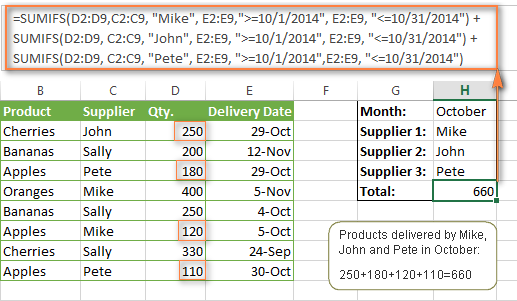
Example 2. SUM & SUMIFS with an array argument
I've tried to explain the essence of this approach in the SUMIF example, so now we can simply copy that formula, change the order of arguments (as you remember it is different in SUMIF and SUMIFS) and add additional criteria. The resulting formula is more compact than SUMIFS + SUMIFS:
=SUM(SUMIFS(D2:D9,C2:C9, {"Mike", "John", "Pete"}, E2:E9,">=10/1/2014", E2:E9, "<=10/31/2014"))
The result returned by this formula is exactly the same as you see in the screenshot above.
Example 3. SUMPRODUCT & SUMIFS
As you remember, the SUMPRODUCT approach differs from the previous two in the way that you enter each of your criteria in a separate cell rather that specify them directly in the formula. In case of several criteria sets, the SUMPRODUCT function won't suffice and you will have to employ ISNUMBER and MATCH as well.
So, assuming that the Supplies Names are in cells H1:H3, Start Date is in cell H4 and End Date in cell H5, our SUMPRODUCT formula takes the following shape:
=SUMPRODUCT(--(E2:E9>=H4), --(E2:E9<=H5), --(ISNUMBER(MATCH(C2:C9, H1:H3,0))), D2:D9)
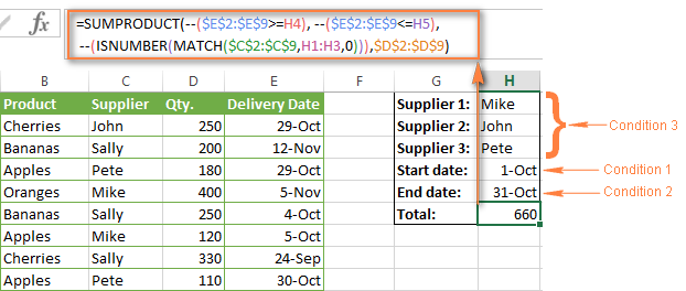
Many people wonder why use double dash (--) in SUMPRODUCT formulas. The point is that Excel SUMPRODUCT ignores all but numeric values, while the comparison operators in our formula return Boolean values (TRUE / FALSE), which are non-numeric. To convert these Boolean values to 1's and 0's, you use the double minus sign, which is technically called the double unary operator. The first unary coerces TRUE/FALSE to -1/0, respectively. The second unary negates the values, i.e. reverses the sign, turning them into +1 and 0, which the SUMPRODUCT function can understand.
I hope the above explanation makes sense. And even if it doesn't, just remember this rule of thumb - use the double unary operator (--) when you are using comparison operators in your SUMPRODUCT formulas.
Using Excel SUM in array formulas
As you remember, Microsoft implemented the SUMIFS function in Excel 2007. If someone still uses Excel 2003, 2000 or earlier, you will have to use a SUM array formula to add values with multiple AND criteria. Naturally, this approach works in modern versions of Excel 2013 - 2007 too, and can be deemed an old-fashioned counterpart of the SUMIFS function.
In the SUMIF formulas discussed above, you have already used array arguments, but an array formula is something different.
Example 1. Sum with multiple AND criteria in Excel 2003 and earlier
Let's get back to the very first example where we found out a sum of amounts relating to a given fruit and supplier:

As you already know, this task is easily accomplished using an ordinary SUMIFS formula:
=SUMIFS(C2:C9, A2:A9, "apples", B2:B9, "Pete")
And now, let's see how the same task can be fulfilled in early "SUMIFS-free" versions of Excel. First off, you write down all the conditions that should be met in the form of range="condition". In this example, we have two range/condition pairs:
Condition 1: A2:A9="apples"
Condition 2: B2:B9="Pete"
Then, you write a SUM formulas that "multiplies" all of your range/condition pairs, each enclosed in brackets. The last multiplier is the sum range, C2:C9 in our case:
=SUM((A2:A9="apples") * ( B2:B9="Pete") * ( C2:C9))
As illustrated in the screenshot below, the formula perfectly works in the latest Excel 2013 version.
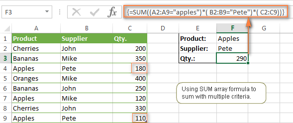
Note. When entering any array formula, you must press Ctrl + Shift + Enter. Once you do this, your formula gets enclosed in {curly braces}, which is a visual indication that an array formula is entered correctly. If you try typing the braces manually, your formula will be converted to a text string, and it won't work.
Example 2. SUM array formulas in modern Excel versions
Even in modern versions of Excel, the power of the SUM function should not be underestimated. The SUM array formula is not simply gymnastics of the mind, but has a practical value, as demonstrated in the following example.
Suppose, you have two columns, B and C, and you need to count how many times column C is greater than column B, when a value in column C is greater or equal to 10. An immediate solution that comes to mind is using the SUM array formula:
=SUM((C1:C10>=10) * (C1:C10>B1:B10))
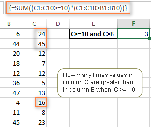
Don't see any practical application to the above formula? Think about it in another way : )
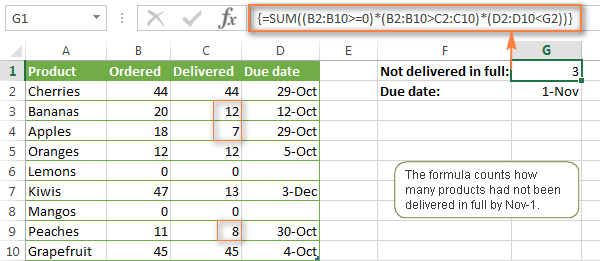
Suppose, you have the orders list like shown in the screenshot below and you want to know how many products have not been delivered in full by a given date. Translated into Excel's language, we have the following conditions:
Condition 1: A value in column B (Ordered items) is greater than 0
Condition 2: A value in column C (Delivered) in less than in column B
Condition 3: A date in column D (Due date) is less than 11/1/2014.
Putting the three range/condition pairs together, you get the following formula:
=SUM((B2:B10>=0)*(B2:B10>C2:C10)*(D2:D10<G2))
Well, the formula examples discussed in this tutorial have only scratched the surface of what Excel SUMIFS and SUMIF functions can really do. But hopefully, they have helped pointing you in the right direction and now you can sum values in your Excel workbooks no matter how many intricate conditions you have to consider.
 by
by
666 comments
Hello,
SUMIF or SUMIFS function add the values specified in 'sum_range'. Usually 'sum_range' should be a row or column of values.
What if the 'sum_range' is a table of array. I mean if quantity of fruits supplied every day is tabled, I want to add quantity of apples supplied in a calendar week, for example CW18. Here 'sum_range' would be "C1:I9". Will It possible to have simple syntax for such summation?
Hi, I have a formula
SUM(SUMIFS('File Name'!D:D,'File Name'!$C:$C,{131,132,133,138}))
that works beautifully when the source file is open but gives me the #VALUE error when it is closed.
Is there a way to rewrite it so that I use only the SUM and IF functions, hopefully avoiding the error?
thanks dears,
could you please help me with multiple (or) conditions in multiple columns
i.g:
SUMIFS(A1:A10,B1:B10,{"Mike","John"},C1:C10,{"Apple","Orange"},D1:D10,"",...)
is this can work in somehow, I try but its give unreal result (Less than the actual) "it seems like the excel is calculating the second (or) condition based on the filtered data in the first (or) condition.
thanks in advanced :),,
hi,
i want to ask
how about if we use criteria (A1:G1)
Hello,
i want to learn below farmula, kindly teach me in detail and example.
SUM(IF(logical_test,[value_if_true],[value_if_false])
Thanks - was struggling with SUMIF and AND together - this explained it clearly and concisely and my report now does what I want it to do.
I want to sum a range to be identified (ex: I have multiple case Id's in which I need to sum the age of the same case id's). Any find formula available.
Example
Case ID Hold Age
10241993 1342.87
10241993 0.02
10241993 126.38
10241993 0.01
10505177 144.04
10505177 18.83
10505177 117.7
... might be nice to point out that the ranges cannot be in adjacent worksheets within a workbook, but must be on the same sheet as the cell in which the formula is entered. I've been trying for an hour to find out what's wrong with my SUMIFS using the sum range and one of the two criteria ranges on another worksheet in the workbook. Always got a 0. Then I moved it all to the same worksheet and it worked fine. Waste of an hour, though...
Hi Dave,
In fact, the sum range and criteria ranges can be on different worksheets provided that all the ranges are of the same size. I've just tested a simple formula like =SUMIFS(Sheet1!A1:A4, Sheet2!A1:A4, "a", Sheet3!A1:A4, "b") and it worked just fine.
I am trying to obtain a year to date utility total using this sumifs formula.
=SUMIFS(cost,meter,$B7,service,$C7,period,"<=$M$1",year,$I$6)
Where range names are
cost = total invoice
meter = the meter number
service = type of utility (gas, water, electricity)
period = the accounting month January - December
year = 2015 or 2016
Thus, the report contains data for all periods 1 - 12 but I want a year to date for any month end (e.g. March would include periods 1, 2, and 3).
Any ideas would be appreciated.
Thanks
I managed to find a solution to my earlier query. I used the sumproduct function and it works perfectly. Irrespective of this, I'd still be interested to know why the sumifs function gives out an error. Regards Charles
I'm trying to use the sumifs function in the last column of a Table (Table1) with a Header Title "Total". Want I need is to add cells of each row based on part of their header title. The first header title within Table1 is "Country", while the other header titles include an abbrev. of the name of each month in the year (i.e. Jan, Feb, etc.). For instance, the header title of B2 is "No of Ships - Jan", C2 is "No of Ships - Feb" and so on until - Dec. The formula is in the rightmost row with a Header Title = "Total". I want to add the No of Ships from x month to y month (x & y being two numeric values inserted by a user outside of the table. Therefore I first started out by using the following formula: =month(datevalue(right(Table1[[#Headers],[No of Ships - Jan]:[No of Ships - Dec]],3)&"1")) which works fine when pressing F9 as the resulting value = 1,2,3..12. However when I try to incorporate the array into the sumifs function, I get an error. Here's the first part of the formula placed in n3:
=sumifs(b3:m3,month(datevalue(right(Table1[[#Headers],[No of Ships - Jan]:[No of Ships]],3)&"1")),">="&A1),... A1 = 5 (meaning start adding from May). If I can get the first part to work, I would then continue the sumifs with the same criteria but based on B1 value (say = 8) being the last month to take into account (in other words add those cells from May to August only). I'd appreciate your help and guidance. (Note that the above is only a simplified version of Table1, which actually incorporates other Header Titles but do not include the month name). Thanks Charles
DATE A B C
01-01-16 999.9 2548.75 2510
01-01-16 1982.7 522.15 0
01-01-16 440.9 0 54
01-01-16 535.5 294.95 0
02-01-16 274.4 0 19
02-01-16 697.5 313.5 0
02-01-16 690.3 179.25 120
03-01-16 158.16 153.8 0
03-01-16 207.5 0 560
04-01-16 1034.1 354.2 0
04-01-16 0 1165.5 8600
04-01-16 180.3 27 0
04-01-16 329.4 665.1 0
Please any one can help me.. i want to total date wise of "A" , "B" AND "C".
Please suggest me how can i total this data..
Hi MANOJ KUMAR,
You should use the following array formulas to sum the values for date 01-01-16:
to sum the "A":
{=SUM(B1:B10 * (A1:A10 = DATE(2016, 1, 1)))}
to sum the "B":
{=SUM(C1:C10 * (A1:A10 = DATE(2016, 1, 1)))}
to sum the "C":
{=SUM(D1:D10 * (A1:A10 = DATE(2016, 1, 1)))}
where
"DATE" values are in A1:A10
"A" values are in B1:B10
"B" values are in C1:C10
"C" values are in D1:D10
To enter this formula press CTRL+SHIFT+ENTER.
I think the SUMIF is exactly what I need - but, I want to find matches in column 1 and 2 (names for example) and then when there is a match - check the third column for a value and place the sum of the values in the third column. If somebody can help I would SO appreciate it..
Hi Beth,
You can use the array formula to solve this task.
For example:
{=SUM(C2:C10 * (A2:A10 = "Text1") * (B2:B10 = "Text2"))}
where
The values are in C2:C10.
The column 1 names are in A2:A10.
The column 2 names are in B2:B10.
To enter this formula press CTRL+SHIFT+ENTER.
Hi Svetlana
Column A: Project ref
Column B: Total hours on Project in one day
Column C: Total hours on one project overall
Rows = Days of the week
Column A consists of multiple reference numbers which repeat if a project is worked on for more than one day, but not necessarily on consecutive days. I want to be able to cumulatively add the total hours worked on a project over multiple days using a sumif calculation. For example i would like the total number of hours worked on project ref 222 over several non consecutive days in one month. The project ref range is large and therefore i do not want to specify "222" in the criteria but all instances where a reference number is repeated in the ref column.
Can you please help.
Thanks
Hi Petros,
You should use the following array formula:
{=SUM(B2:B10 * (A2:A10 = "222"))}
where
"Total hours on Project in one day" is in B2:B10
"Project ref" is in A2:A10
To enter this formula press CTRL+SHIFT+ENTER.
Thanks you all.
hello,
Please send me Formulas
Exp.
this is pan number list
AAAPA1234A
AAACA1234A
AAAHA1234A
When Pan number Four letter is P=2
otherwise=1
AAAPA1234A 1
AAACA1234A 2
AAAHA1234A 2
AAAFA1234A 2
ABCPA1250A 1
Please send me formula....
Hi SACHIN,
Please try the following formula:
=IF(MID(A1, 4, 1)="P", 1, 2)
Hello,
I am trying to say sum a column which does not equal a range of criteria in one criteria range.
This is an example of my criteria range & criteria, but I cannot get it to work: (The actual formula is more complex and much longer)
Data!$A:$A,""I have to put SUM() around the SUMIFS() which works, but not when I add ""&
Any suggestions?
Thanks
Hi Victoria,
To be able to assist you better please describe your task in more detail.
I want to Use SUMIF Function in a column where i need to find different values and total it for example:
i want to use sumif formulae like this in n. no of cell
SUMIF(I1:I1000, "6625", K1:K1000)
SUMIF(I1:I1000, "6626", K1:K1000)
SUMIF(I1:I1000, "6627", K1:K1000)
SUMIF(I1:I1000, "6628", K1:K1000)
now how can i rite this in entire cell with different values to search
Dear All
Looking for needy help..
I have to prepare one Status report to My Manager, Actually in my office several consultant working on a daily basis and my boss given to them number of works on a daily basis for example:- A, B , C consultants, Boss has given number of works to them like For A on 21-01-2016 hes has to complete 10jobs and "B" 5Jobs,C" 8. On 22-01-2016 "A" 5,"B"8,"C"10. We want to know how much they completed as on date and how much pending namewsie.
Waiting for positive reply
Thanking you
Hi Alexander,
Please check the below table for the same.
OrderID AgentName Center Qty Sum of Single cell Qty
VI8736656 Amit Kumar Techm Noida 23 5
VI8736685 Rakesh Chand Techm Noida 245 11
VI8736986 Ruby Techm Chennai 23 5
VI8737133 Lokesh Kushwaha Techm Noida 31 4
VI8737537 Seethala Devi L Techm Chennai 234 9
VI8737539 Seethala Devi L Techm Chennai 2 2
VI8737682 Md Rafee Alam Techm Noida 134 8
VI8738184 Komal Singh Techm Noida 246 12
VI8738222 Chakshu Jain Techm Noida 309 12
VI8738396 Md Rafee Alam Techm Noida 278 17
VI8738507 Aanchal Techm Noida 245 11
Hello Anand,
Would it be possible for you to email your Excel file to support@ablebits.com?
It is very difficult to see the structure of your data here and tell one column from another.
Hi Guys
Anybody could you help me and can you explain the below formula step by step
Because I am not able to undersand this formula.
please please help me
=SUMPRODUCT(1*MID(H7,ROW(INDIRECT("1:"&LEN(H7))),1))
Hello, Anand,
To help you better, we need a sample table with your data in Excel. You can email it to support@ablebits.com. Please add the link to this article and your comment number.
Hi!
I'm trying to use function SUMIFS to sum up numbers by account (column A), product (column B), year (row 1) and scenario (row 2). But the only thing I get is #VALUE.
Is it possible to at all to use SUMIFS in such cases? Or is there any better function for this purpose?
Hi Melissa,
It is possible, but could you send a sample worksheet to support@ablebits.com? Please include a link to this blog post and your comment number.
We'll do our best to assist you.
Hi Irina!
Thank you! I think I have figured out it in a slightly different way:-) But I'll keep in mind your site!
/Melissa
I almost have this figured out...Help please.
I have a simple list of ages and zip codes. Ages are broken into categories as such:0-5, 6-11, 12-18, Adult, Adult +. The zip codes and ages need to be tallied. I need to know how many of each age participated and I need to know from what zip codes these folks have come from. Here is an example...
A B C D E F G H
55 ADULT 97478 0 0 0 0 0
56 ADULT 97402 0 0 0 0 0
57 3 97402 1 0 0 0 0
58 3 97402 1 0 0 0 0
59 6 97402 0 1 0 0 0
AGE 0-5 6-11 12-18 Adult Adult +
TOTALS
ZIP CODE 97402 97404 97405 97478
TOTALS
The formula in D57 is =IF(AND(B60>0,B60<6),"1","0") This formula does exactly what I ask it to do. However, I am unable to sum each column, The formula does not recognize text, and I am not sure what to do with The zip codes. Can you help?
Hi Shelly,
You can use the COUNTIF or COUNTIFS functions, please see the following articles for more details:
COUNTIF in Excel
How to use COUNTIFS
If you need to get a unique list of ZIP codes for each age group, then please follow these steps:
- Create a copy of your worksheet;
- Add a helper column J, enter the following formula into its first cell:
=IF(AND($B1>=0,$B1<=5),"0-6",IF(AND($B1>=6,$B1<=11),"6-11",IF(AND($B1>=12,$B1<=18),"12-18",IF($B1="Adult","Adult","Adult+"))))
- Copy it down the column;
- Run our Combine Rows Wizard add-in
- Use column G as the key column, choose to combine the unique values in the column with the ZIP codes and separate them with a comma.
I have a budget workbook I'm working on.
We have expenses assigned to Categories, Types. They are allocated in Programs. In one worksheet, columns have an array formula to sum up data from an expense page
{=SUM(SUMIFS('Dollar Data'!$E$2:$E$352,'Dollar Data'!$A$2:$A$352,$A10,'Dollar Data'!$C$2:$C$352,D$154:D$173))}
Dollar Data A is Type,
Dollar Data C is Category,
Categories are allocated to Programs (multiple columns).
Right now all of a Category is assigned to a Program, and we want to assign it proportionally. Is it possible to tweak the array formula to use a percentage? We could specify it next to our Category Criteria in D$154:D$173, e.g. E$154:E$173.
as a simplified example:
e.g. Program A = Break Room Program B = Parties.
Program A Prcnt Program B Prcnt
Silverware 60 Silverware 40
(Type is Knives, Forks, Spoons, all added together into Silverware by the array formula).
Excellent, many thanks for your help, the community appreciates !
I'm trying this formula but its not working on my sheet
=SUMIFS(I10:I88,G10:G88,"AGO - PETROL",H10:H88,"874")
My table has all the columns but when pressing enter key to get the
result comes a #value . Can anyone help me knowing the problem?
Control + Shift + Enter instead of Enter to enter it as an array formula...
Very helpful article, and it got me almost all the way to a solution, but now I am stuck because I can't get the SUMIFS function to apply as an array formula. Right now I am using the following (=SUMIFS($J2:$J152, $L2:$L152, L2, $E2:$E152, E2). I need the values with the $ to stay static and for the values without the $ to move as the formula is applied, but with SUMIFS it doesn't seem to work the way normal formulas work. How can I get SUMIFS to respect the $?!
Thank you.
I believe you would not include the parentheses around the very outside around the =. you would enter the formula, and hit Control + Shift + Enter to create the array formula...
Hi,
Sorry if I missed this in your post. I am using the below formula:
=SUM(IF(FREQUENCY(A2:A367,A2:A367)>0,1))+SUM(IF(FREQUENCY('Sheet2'!A2:A367,'Sheet2'!A2:A367)>0,1))
This gives me a total unique count from two separate sheets. However I now want to count the unique values with criteria attached. I tried the following:
=SUMIFS(IF(FREQUENCY(A2:A367,A2:A367)>0,1),B2:B4367,">="&Settings!B6, B2:B367,"0,1),Sheet2!B2:B367,">="&Settings!B6,Sheet2!B2:B367,"<="&Settings!B5)
However it only comes up with a #Value! error. I feel as though I am missing something obvious with the structure of the nested IF within the SUMIF but I can't see it.
Thanks for any help :)
Just as an update, I attempted nesting the IF functions against the criteria and against the range manually but I was still unable to retrieve a functional result.
Hello, Michael,
To find an error in the second formula we need to see your data. You can send us a small sample table with your data in Excel to support@ablebits.com. Please include the link to this article and the number of your comment.
Thank you for your reply. I worked it out as follows:
=SUM(IF(FREQUENCY(IF(CUKD>=Settings!B8,IF(CUKT"",MATCH("~"&CUKT,CUKT&"",0))),ROW(CUKT)-ROW('Current Year UK'!A2)+1),1))+SUM(IF(FREQUENCY(IF(CUSD>=Settings!B8,IF(CUST"",MATCH("~"&CUST,CUST&"",0))),ROW(CUST)-ROW('Current Year US'!A2)+1),1))
The structure was flawed in that the criteria was being applied but not as part of the SUMIF function, at least not correctly. It was far easier instead to simply specify nested IF functions as above and push as an Array. The named ranges are simply just to reduce loading time for adjusted ranges, it will eventually become a requirement to use SQL to perform the same function, but by that point I think I will migrate from Excel altogether.
After much "Googling", this is the best treatment of this subject that I saw.
Mega-thanks to you Svetlana.
I want to use the sumifs formula but for a "text" in the sum_range. Is this possible? I have a list of products or tours, by date with a particular guide or guides. I am using sumifs to get the criteria of the date and guide name but the resulting answer is in text (product), not a numerical value. What would be the formula for sumifs for a text value?
Thanks in advance!
Hello, Robin,
It's not possible to sum text with SUMIF. The cells must contain numbers, names, arrays, or links to numbers. Empty cells and text cells are skipped.
Hi There are subject codes and grades scattered in various columns & rows in excel sheet . how can i extract counted grades & code in one cell of excel sheet jointly. FOR EXAMPLE CODE 30 GRADE A1 I WANT TO KNOW 4 Columns is there for formula help automatically count and write whole sheet how many code 30 get A1 grade manually count code 30 grade A1 is 4.please solve my problem.
chart is given below.
NAME CODE GRD CODE GRD CODE GRD CODE GRD
RAM 30 A1 41 A1 30 A1 41 A1
SHYAM 41 A1 30 A1 41 A1 30 A1
Advance thanks
As soon as possible please give reply
Hi, There are subject codes and grades scattered in various columns & rows in excel sheet. how can i extract counted grades & codes in one cell of excel sheet. For example code 30 grade A1 how to count how many 30 code get A1 grade manually count code 30 A1 grade is 4. but i want to formula help automatically count and write.Please help me. pandey5375@gmail.com
chart is given below.
NAME CODE GRD CODE GRD CODE GRD CODE GRD
RAM 30 A1 41 A1 30 A1 41 A1
SHYAM 41 A1 30 A1 41 A1 30 A1
Hi,
in my spreadsheet a column has date values. eg
F20 = 1/1/2016, G20 = 120
F21 = 1/2/2016, G21 = 80
F22 = 1/5/2016, G22 = 120
F23 = 1/6/2016, G23 = 100
F24 = 1/9/2016, G24 = 200
and it has been entered so on.
I'm querying F column for the cell having latest date value. here F24 has.
then i want to retrieve cell G24 value in corresponding row, here G24 = 200 and want to store in Cell E2.
Now as i enter new data in F25:G25, F26:G26 and so on Cell E2 should update automatically as per latest date entry in F column.
please guide here how to achieve this in Excel 2013.
Try using max(F:F) as your criterion.
can sombody tell me
how is use this
=sumproduct(K1:K10)*(L1:L10)*(O1:O10)*(P1:P10)*(B1:B10={"A","B","C")*(1)
XAX
THANK'S MAM FOR PROVIDING FANTASTIC FORMULAS TIPS............
Hello Everyone,
...Im a bit stuck on a formula. I hope I can find a solution
I have to create a price list for a bunch of products that have up to 3 different discount prices available depending on the quantity..
How do I write the formula so that the correct amount will appear?
So for example :
When buying :
- a quantity of 49 apples or less, the cost of each apple would be .20 cents each.
- a quantity of 50 - 75 apples, the cost of each apple is .10 cents
- a quantity of 76 - 120 apples, the cost of each apple becomes .5 cents...
Thank You!
Jean
=IF(A176,0.05,0.1))
Where A1 is your product quantity. Just copy down against all products.
Though, if you are discounting, you would be better off listing the full price and applying a discount rate based on cell values held elsewhere.
Dear Svetlana,
I am struggling with the following formula. I would like to sum a1:a200 if b1:b200 contains patrial text match "CMCM*" AND "CMME*" AND "CMCO*", but also if c1:c200 matches with {'sheet2'!a1:a50} (so any match in that range)
I came up with =SUMIFS($A$1:$A$200;$B$1:$B$200;{"CMCM*";CMME*";"CMCO*"};$C$1:$C$200;{'sheet2'!A1:A50}).
The issue in this is that it does sum some of the matches, but I want to sum all possibilities.
Could you help me find the right formula? I hope it is possible.
Best regards, Bram
I found out how it works. The following formula does the trick:
=SUMPRODUCT(--(ISNUMBER(MATCH($C$1:$C$200;'sheet2'!$A$1:$A$50;0)));--(ISNUMBER(MATCH($B$1:$B$200;Formula!$A$1:$A$3;0)));$A$1:$A$200)
where Formula!$A$1:$A$3 contains the partial match criteria.
please some one explain this to me
=1-SUMIFS(AG:AG,AB:AB,AB181,AE:AE,"No")/(1440*224)
Sumif does not consider case because in the examples, bananas matches Bananas.
However, does sumif match the entire cell's text? I.E. if the text being searched for was "banana" would it match "Bananas"?
I think not as I tried it in one of my spreadsheets. In order to match "grape" and "grapefruits" I used "grape*", but my results are not what I expected even then.
I got zero (for the sumif) when I didn't use the '*' wildcard, but the non-zero number I got using the wildcard(s) does not match the number I get when I use the find (button) to look for "grape" ("find" the button, finds subsets of text within the cells so it does find both Grapes and Grapefruits) and then I used "=sum()" of the found text's associated number cell).
What's even more interesting is that the non-zero number I got doesn't match the "=sum()" of ANY combination of the cells I want sumif'd!
For this sumif case it's only four cells of >400 to be summed, but there are other cases where I will need a hundred out of thousands of cells, so I'd like to figure this out.
To figure this out, how can one determine which cells a sumif is summing?
(I.E. what is it doing so I can make it do-right?)
(I don't know if it matters but I'm using Office 2011 on Mac OSX.)
I found out that selecting the cell with the formula and then going to the Formulas tab (Excel 2011) and clicking on Trace Precedents draws arrows from the cells feeding the formula. Clicking it again should show the next prior cell feeding the formula. It worked for my =cell+cell+cell+cell formula, but for my sumif it drew one arrow from the formula to the top cell of the search for text cell, ie, D1. That's it. I can't even find any cell with the number the sumif gives (1076.35).
By the way, in my case the numbers to be sumif'd are 1244.24 + 361.80 + 1047.35 + 433.35 = 3086.74, but the sumif result is 1076.35.
Hi,
The following formulas cannnot work. I tried removing (GL!$BG:$BG,CY$1:CY$2), it works. Apparently, it can't seems to add more than 1 range of cells in the formulas below. Is there any solutions to this? Appreciate your help.
=SUMPRODUCT(SUMIFS(OFFSET(GL!$D:$D,0,MATCH(CY$9&"-"&'Grp PnL'!$T$3,GL!$D$1:$BN$1,0)-1),GL!$D:$D,'Grp PnL'!$D71,GL!$C:$C,CY$3:CZ$6,GL!$BG:$BG,CY$1:CY$2))
Hello, Jacqueline,
It's hard to find the error without looking at your data. Please send us a small sample table with your data in Excel to support@ablebits.com.
Summing Across a Row?
I thought this would be relatively simple but I cannot figure a way to do it (granted I am not a superuser - yet). Here is the problem:
Given a ROW of data as follows:
A,3,B,6,A,5,A,2,B,7
I want to sum all the values which follow an A and then sum all the values which follow a B. So output would be in two cells one for A values which would equal 10 and the other for B values which would equal 13.
I tried using SUMIF array formula but maybe that is not possible. I would hate to have to use a combination of simple IFs as the rows are long and there are a lot of them so thought array formula might help. Any suggestions?
Hello, Eddie,
If the number of values in rows is fixed, you can use this formula:
=SUM(F12*IF(E12="A", 1, 0), H12*IF(G12="A", 1, 0),J12*IF(I12="A", 1, 0),L12*IF(K12="A", 1, 0),N12*IF(M12="A", 1, 0))
=SUM(F12*IF(E12="B", 1, 0), H12*IF(G12="B", 1, 0),J12*IF(I12="B", 1, 0),L12*IF(K12="B", 1, 0),N12*IF(M12="B", 1, 0))
If the rows length varies you need this array formula:
{=SUM(IF(OFFSET(B1:K1, 0, -1) = "A", 1, 0) * IF(ISNUMBER(B1:K1), B1:K1, 0))}
{=SUM(IF(OFFSET(B1:K1, 0, -1) = "B", 1, 0) * IF(ISNUMBER(B1:K1), B1:K1, 0))}
Hi,
Some thing is not right in my function ( ie 'BIN DETAIL'!Y3:Y1000,{"";"="&today()} ) it is giving me the total of one criteria instead of two creteria)
=sum(SUMIFS('BIN DETAIL'!H3:H1000,'BIN DETAIL'!I3:I1000,"",'BIN DETAIL'!X3:X1000,""&"rej",'BIN DETAIL'!Y3:Y1000,{"";"="&today()}))
Can you provide me with a basic difference between SUMIF and SUMIFS?
Thank you.
Hello Julie,
SUMIF adds up cells based on 1 criterion, SUMIFS allows for multiple criteria.
in the first chart (product, supplier).. is there a way to know for example the number of total "Apples" if I leave blank in "supplier"? in other words: if i choose a specific product and supplier, i use sumifs. BUT if i want to leave blank in supplier or product, and want to get the total (would be: blank criteria = consider all). how can I do this? thanks!!!
I would like to use the SUMIFS formula but in the criteria I would like to use the "inverse" of a criteria. For example using your example above I would to sum all items that are NOT supplied by John. This is because sometimes to specify all the criteria would be laborious!!
please help me with this
i need a formula that says
ex.
A2 B2 C2 D2
10 4 40% Not ok
if the result of c2 is equal or less than 50% put "ok" otherwise not ok. thank you very much and i will really appreciate your response.
Hi, Please see spreadsheet below. what i want to do is: Calculate the total of apples in column 1 but only if column 2 is yes.
fruit sold
apples yes
banana no
pineapple yes
pear yes
litchi no
total sold total not sold
apples
banana
pineapple
pear
litchi
Hi - I just can't figure out what to do! This is my first time using SUMIFS ... and I can't get the right answer.
Raw Data
Column A - List of Names
Column C - No. of Hours
Column D - Hour Type (Class, Coach, Administrative, etc.)
SUMMARY
Column H - Name Entered
Column J -- Need to use SUMIFS to total all hours (Column C) for the name in (Column A) that equals the name listed in Column H as long as that Hour Type is NOT "Administrative"
Thanks!!!