In this article you'll find out how to add comments to Excel cells, show, hide and delete them. You'll also learn how to insert a picture in a comment and make your cell note more eye-catching by changing its font, shape and size.
Suppose you have received an Excel document from another person and want to leave your feedback, make corrections or ask questions about the data. You can easily do this by adding a comment to a particular cell in the worksheet. A comment is often the best way to attach additional information to a cell because it doesn't change the data itself.
This tool can also come in handy when you need to explain formulas to other users or describe a certain value. Instead of entering text description you can insert a picture into a comment.
If you want to know more about this Excel feature, go ahead and read this article!
Add comments in Excel
First I should say that the ways of inserting text and picture notes are different. So let's begin with the easiest of two and add a text comment to a cell.
- Select the cell that you want to comment on.
- Go to the REVIEWtab and click on the New Comment icon in the Comments section.
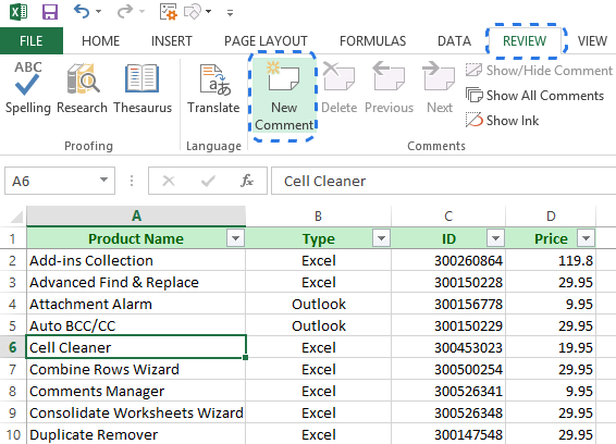
Note. To perform this task you can also use the Shift + F2 keyboard shortcut or right-click on the cell and choose the Insert Comment option from the menu list.
By default, every new comment is labelled with the Microsoft Office user name, but this may not be you. In this case you can delete the default name from the comment box and enter your own one. You can replace it with any other text as well.
Note. If you want your name to always appear in all your comments, follow the link to one of our previous blog posts and find out how to change the default author name in Excel.
- Enter your remarks in the comment box.
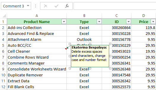
- Click on any other cell in the worksheet.
The text will go, but the little red indicator will remain in the upper-right corner of the cell. It shows that the cell contains the comment. Just hover the pointer over the cell to read the note.
Tip. To see who has commented on a particular cell, take a look at the Excel status bar.
How to show / hide Excel cell notes
I've just mentioned above how to view a single comment in the worksheet, but at some point you may want to display all of them at once. Just navigate to the Comments section on the REVIEW tab and click on the Show All Comments option.
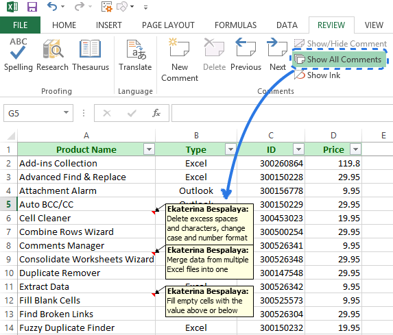
One click and all the comments in the current sheet are displayed on the screen. After reviewing the cell notes, you can hide them by clicking Show All Comments again.
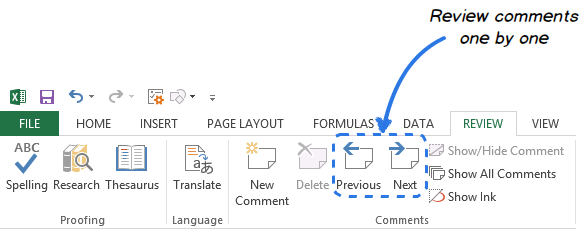
If you have a lot of comments in the spreadsheet, showing all of them at a time can complicate your perception of the data. In this case you can cycle through the comments using the Next and Previous buttons on the REVIEW tab.
If you need a single comment to stay visible for a while, right-click on the cell with it and choose Show/Hide Comments from the menu. You can also find this option in the Comments section on the REVIEW tab.
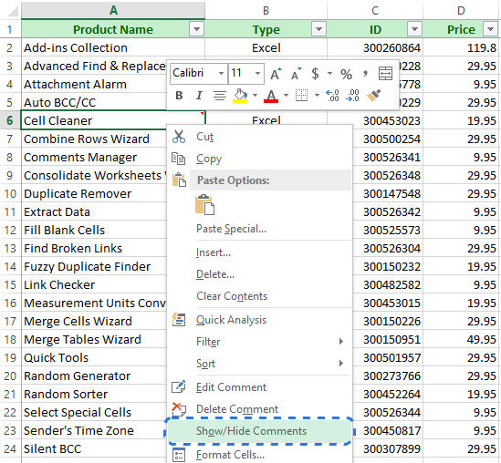
To put the comment out of sight, right-click on the cell and select Hide Comment from the menu or click on the Show/Hide Comments option on the REVIEW tab.
Make your comment look good
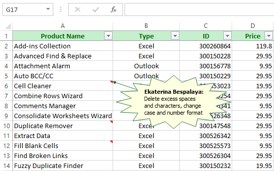
The rectangular shape, pale yellow background, Tahoma 8 font... A standard comment in Excel looks rather boring and unattractive, doesn't it? Fortunately, with a little bit of imagination and skill, you can make it more eye-catching.
Change the font
The font of an individual comment is very easy to change.
- Select the cell that contains the comment you want to format.
- Right-click and choose the Edit Comment option from the menu.
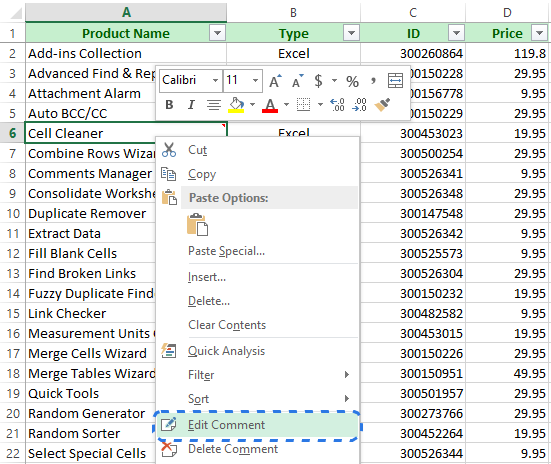
You will see the comment box selected with the flashing cursor inside it.
There are two more ways to select the comment. You can either go to the Comments section on the REVIEW tab and click on the Edit Comment option or press Shift + F2.
- Highlight the text where you want to change the font.
- Right-click on the selection and choose the Format Comment option.
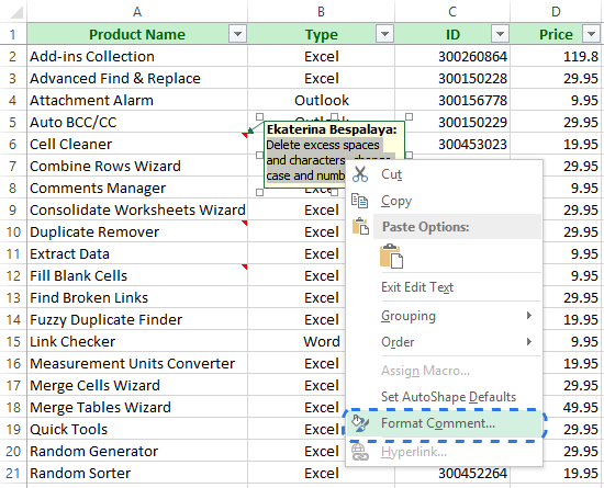
The Format Comment dialog window will appear on your screen. Here you can pick the font, font style or size that you like, add different effects to the comment text or change its color.
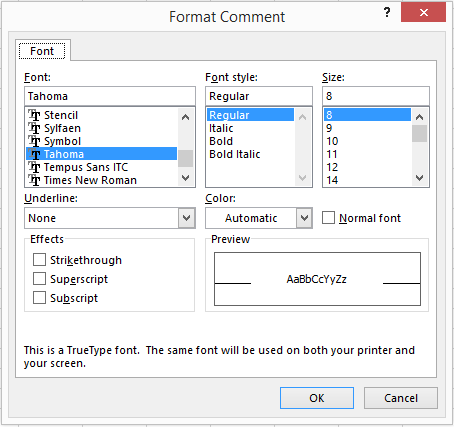
- Make changes that you want and click OK.
If you are sick and tired of changing the font size of each single comment, you can apply it to all cell notes at once by changing the settings in your Control Panel.
Note. This update will affect Excel comments, as well as tooltips in other programs.
Change comment shape
If you want to use a different comment shape instead of the standard rectangle, first you need to add a special command to the Quick Access Toolbar (QAT).
- Open the Customize QAT drop-down menu and choose the More Commands option.
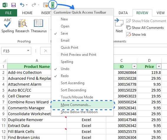
You will see the Excel Options dialog window on your screen.
- Pick Drawing Tools | Format Tab from the Choose commands from drop-down menu.
- Choose Change Shape in the list of commands.
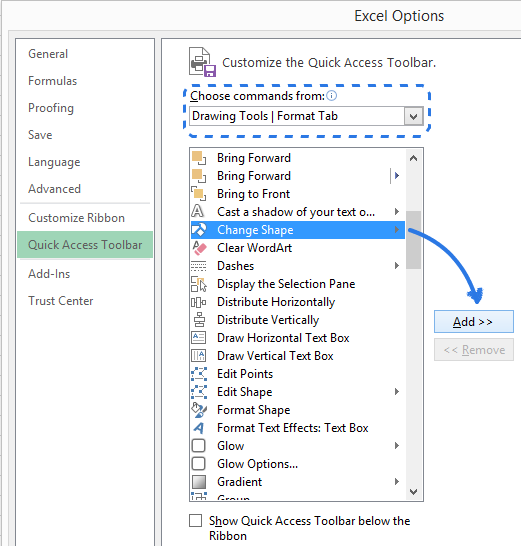
- Click Add and then OK.
The Change Shape icon is added to the QAT in the top-left corner of the Excel window, but it is grayed out. To enable the icon, click on the comment border using the four-headed arrow.
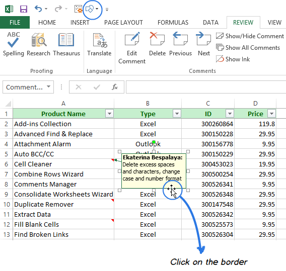
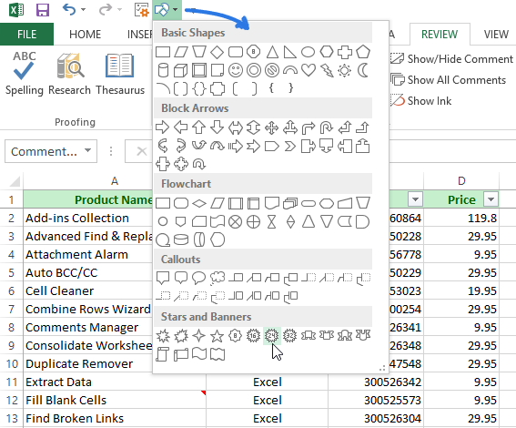
When the option becomes available, open the Change Shape drop-down list and choose the shape you want.
Resize a comment
After you've changed the comment shape it can happen that the text doesn't fit the comment box. Do the following to solve this problem:
- Select the comment.
- Hover the pointer over the sizing handles.
- old down the left mouse button and drag the handles to change the comment size.
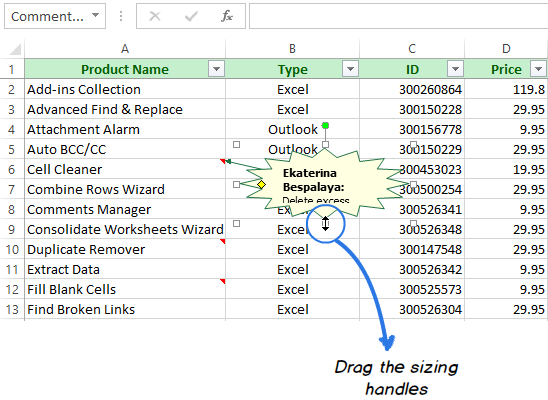
Now when your comment has its individual style, hardly it will be ignored.
How to copy comments to other cells in Excel
If you want the same comment in multiple cells of your worksheet, you can copy and paste it in other cells without changing their content.
- Select the commented cell.
- Press Ctrl + C or right-click and choose the Copy option.
- Select the cell or the range of cells where you want to have the same comment.
- Navigate to the Clipboard group on the HOME tab and open the Paste drop-down list.
- Click on the Paste Special option at the bottom of the menu.
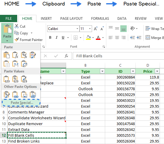
You will get the Paste Special dialog box on the screen.
Note. You can skip steps 4 - 5 and use the Ctrl + Alt + V keyboard shortcut to display the Paste Special dialog.
- Select the Comments radio button in the Paste section of the dialog window.
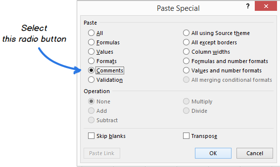
- Click OK.
As the result, only the comment will be pasted into all the selected cells. If any cell in the destination area already has a comment, it will be replaced with the one you paste.
Delete comments
If you no longer need a comment, just follow the steps below to get rid of it in a second:
- Select the cell or cells that contain comments.
- Right-click and choose the Delete Comment option from the context menu.
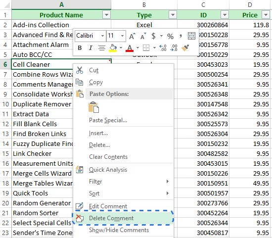
You can also go to the REVIEW tab in the Ribbon and click on the Delete icon in the Comments section to clear the comments out of the selected cell or range.
As soon as you do that, the red indicator will disappear and the cell will no longer contain the note.
Insert a picture in a comment
It's high time to find out how to insert a picture comment in Excel. It may be very helpful when you want other spreadsheet users to have the visual presentation of your data. You can add the pictures of products, company logos, diagrams, schemes or fragments of a map as comments in Excel.
This task will take you some time, but I am sure it will be no problem at all. First let's try to do it manually.
Method 1
- Right-click the cell and choose Insert Comment from the context menu.
Note. In case the cell already contains a note, you need to make it visible. Right-click on the commented cell and choose the Show/Hide Comments option from the menu.
If you don't want any text in your picture comment, just delete it.
- Point to the comment border and right-click on it.
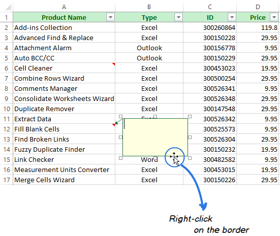
Note. It is important to right-click on the border not inside the comment box since the Format Comment dialog window will have different options in each case.
- Pick the Format Comment option from the context menu.
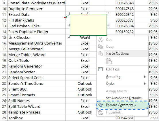
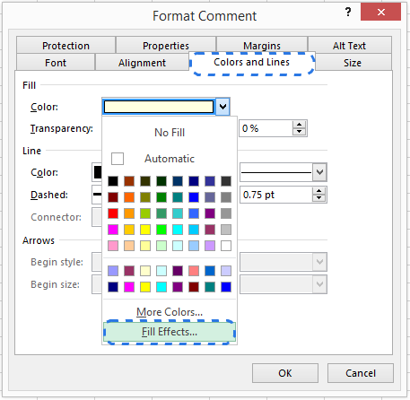
- Switch to the Colors and Lines tab in the Format Comment dialog window.
- Open the Color drop-down list in the Fill section.
- Click on Fill Effects...
- Go to the Picture tab in the Fill Effects dialog.
- Press the Select Picture button to browse for an image file on your computer or on the Web.
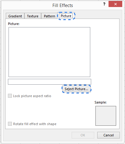
- When you find the necessary image, select it and click Insert.
The image appears in the Picture field of the Fill Effects dialog. To keep the picture proportions, check the box next to Lock Picture Aspect Ratio.
- Close the Fill Effects and Format Comment dialog windows by clicking OK.
Method 2
If you want to speed up the process of adding a picture comment to a cell in your worksheet, use Quick Tools by Ablebits.
Quick Tools for Microsoft Excel is a set of 10 great utilities that can make your daily tasks quicker and easier. Besides adding a picture comment to a cell, these tools can help you with math calculations, filtering data, converting formulas and copying cell addresses.
Now let me show you how Quick Tools can help you insert a picture into a comment.
- Download Quick Tools and install it on your computer.
After the installation the new Ablebits Quick Tools tab appears in the Ribbon.
- Select the cell where you want to add a picture comment.
- Click on the Insert Picture icon on the Ablebits Quick Tools tab and browse for the necessary image file on your PC.

- Just click Open to see the result.
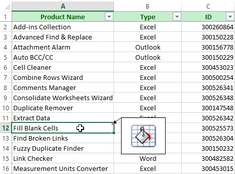
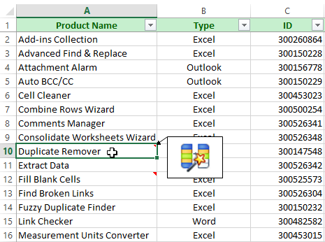
When you rest the pointer on the cell, you'll see the picture you've just inserted in the comment.
Quick Tools also allows you to change the comment shape. First you need to click on the comment border to enable the Change Shape button in the Comment section. Then just pick the shape you like from the Change Shape drop-down list.
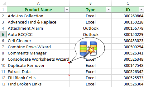
Now your comment will definitely catch everyone's interest because it contains the necessary details and visual support.
I hope after reading this article you will have no problem with adding, changing, showing, hiding, copying and deleting text and picture comments in Excel workbooks. If you have, just leave me a comment here and I'll do my best to help you! :)
 by
by
57 comments
Shbdhdsb
Whether you're a beginner or an advanced user, Excel's versatility and user-friendly interface make it a staple for professionals across various industries.
Learn more about MS Excel in Micro wave computer institute khanna.---- 988500936
Outstanding way of explaining. You have described in detail step by step. It is so helpful. Thank you so much for sharing this useful information.
You can insert a comment in a cell using the Ribbon. By default, when you insert the comments in excel, it will only display the comment indicators in cells.
thanks alot of infformation mantap bet
There use to be a way to add a note within a cell. Not the small triangle method where you have to hover over the note. There use to be a way when you clicked on the cell, it could contain the equation, and you could see text that wouldn't show once you clicked off the cell.
This allowed you to arrow down through cells, see the notes, and not have to hover over the cell. It's been awhile and I can't remember how to do it.
Is there any way to auto copy comment to the cell from another sheet wherever I add in the part number . Cos in my spreadsheet different part number has different requirement . Induvial part has different job scope . So I wanted to auto copy it in the comment ..Possible , pls advice
This is great, however, I would like the picture in the comment to change automatically depending on the content of the cell (Drop-down).
Is this possible?
Nice Post!
Hi, this article is absolutely perfect. good information. thanks for sharing this post .good work
Hello, I'm Bradley Noah. This post is very important information. I really enjoyed this post enough to search for writing this excellent article and helpful post thanks for sharing.
I only saw a little clip from a Google search but I found this was helpful.
Excel 2010, adding a comment is super easy and the same as 2013. ... “Windows User” and that's because the copy of Office is registered to ..
This is very informative and useful post. Thanks for sharing!
You’re a good looking inspiration.
I really informative article its to helpful i really enjoyed its reading this post enough to search high quality clothing manufacturers to helpful post thanks for sharing.
Instead of text, you can show a picture in an Excel comment. Right-click the cell which contains the comment. Choose Show/Hide Comments, and clear any text from the comment. Click on the border of the comment, to select it.
Right-click the cell and then click Insert Comment (or press Shift+F2). If you're using Excel for Office 365, right-click the cell and choose New Note. Type your annotation text. Click outside the ce
Excel displays the Select Picture dialog box, which looks very similar to a standard Open dialog box. Use the controls in the dialog box to locate the picture you want in the comment or note. Select the picture and click the Insert button.
This macro will be used to set photos or images in the background to the comment box from the computer. It will make comments and Excel look more attractive.