The tutorial shows how to make custom Data Validation rules in Excel. You will find a few examples of Excel data validation formulas to allow only numbers or text values in specific cells, or only text beginning with specific characters, permit unique data preventing duplicates, and more.
In yesterday's tutorial we started to look at Excel Data Validation - what its purpose is, how it works, and how to use built-in rules to validate data in your worksheets. Today, we are going to take a step further and talk about the nitty-gritty aspects of custom data validation in Excel as well as experiment with a handful of different validation formulas.
How to create custom data validation with formula
Microsoft Excel has several built-in data validation rules for numbers, dates and text, but they cover only the most basic scenarios. If you want to validate cells with your own criteria, create a custom validation rule based on a formula. Here's how:
- Select one or more cells to validate.
- Open the Data Validation dialog box. For this, click the Data Validation button on the Data tab, in the Data Tools group or press the key sequence Alt > D > L (each key is to be pressed separately).
- On the Settings tab of the Data Validation dialog window, select Custom in the Allow box, and enter your data validation formula in the Formula box.
- Click OK.
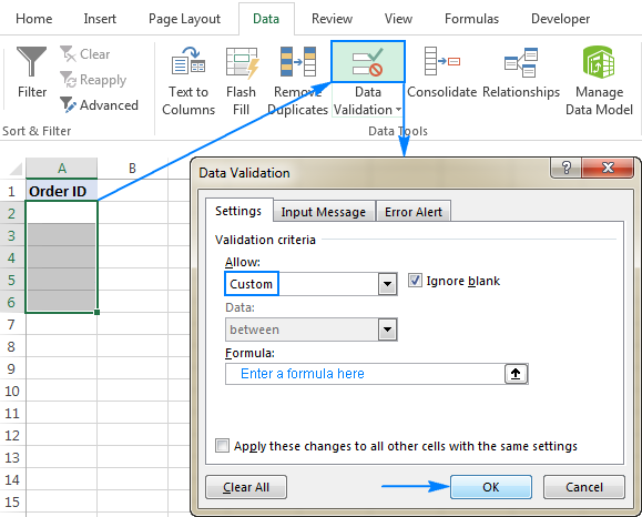
Optionally, you can add a custom input message and Error alert that will show up when the user selects the validated cell or enters invalid data, respectively.
Below you will find a few examples of custom validation rules for different data types.
Note. All Excel data validation rules, built-in and custom, verify only new data that is typed in a cell after creating the rule. Copied data is not validated, nor is the data input in the cell before making the rule. To pin down existing entries that do not meet your data validation criteria, use the Circle Invalid Data feature as shown in How to find invalid data in Excel.
Excel data validation to allow numbers only
Surprisingly, none of the inbuilt Excel data validation rules cater for a very typical situation when you need to restrict users to entering only numbers in specific cells. But this can be easily done with a custom data validation formula based on the ISNUMBER function, like this one:
=ISNUMBER(C2)
Where C2 is the topmost cell of the range you want to validate.
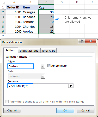
Note. The ISNUMBER function allows any numeric values in validated cells, including integers, decimals, fractions as well as dates and times, which are also numbers in terms of Excel.
Excel data validation to allow text only
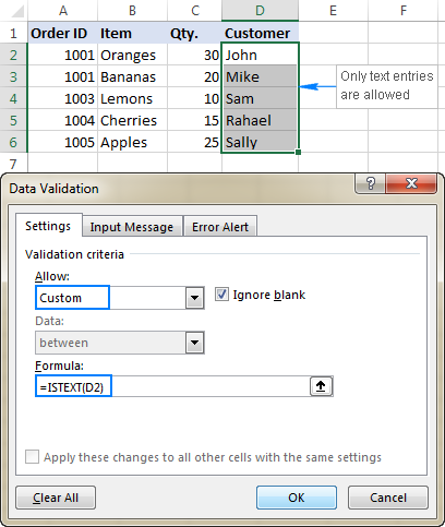
If you are looking for the opposite - to allow only text entries in given range of cells, then build a custom rule with the ISTEXT function, for example:
=ISTEXT(D2)
Where D2 is the uppermost cell of the selected range.
Allow text beginning with specific character(s)
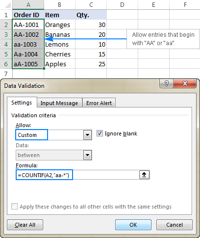
If all values in a certain range should begin with a particular character or substring, then do Excel data validation based on the COUNTIF function with a wildcard character:
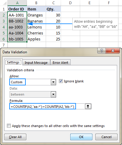
For example, to ensure that all order id's in column A begin with the "AA-", "aa-", "Aa-", or "aA-" prefix (case-insensitive), define a custom rule with this data validation formula:
=COUNTIF(A2,"aa-*")
Validation formula with the OR logic (multiple criteria)
In case there are 2 or more valid prefixes, add up several COUNTIF functions, so that your Excel data validation rule works with the OR logic:
=COUNTIF(A2,"aa-*")+COUNTIF(A2,"bb-*")
Case-sensitive validation formula
If the character case matters, then use EXACT in combination with the LEFT function to create a case-sensitive validation formula for entries beginning with specific text:
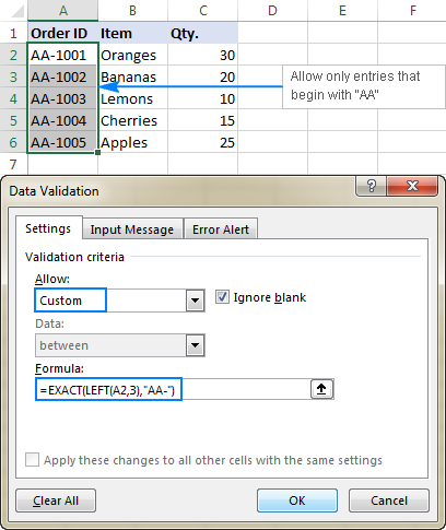
For instance, to allow only those order ids that begin with "AA-" (neither "aa-" nor "Aa-" is allowed), use this formula:
=EXACT(LEFT(A2,3),"AA-")
In the above formula, the LEFT function extracts the first 3 characters from cell A2, and EXACT performs a case-sensitive comparison with the hard-coded substring ("AA-" in this example). If the two substrings match exactly, the formula returns TRUE and the validation passes; otherwise FALSE is returned and the validation fails.
Allow entries containing certain text
To allow entries that contain specific text anywhere in a cell (in the beginning, middle, or end), use the ISNUMBER function in combination with either FIND or SEARCH depending on whether you want case-sensitive or case-insensitive match:
- Case-insensitive validation:
ISNUMBER(SEARCH(text, cell))
- Case-sensitive validation:
ISNUMBER(FIND(text, cell))
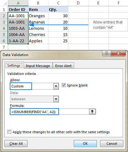
On our sample data set, to permit only entries containing the text "AA" in cells A2:A6, use one of these formulas:
Case-insensitive:
=ISNUMBER(SEARCH("AA", A2))
Case-sensitive:
=ISNUMBER(FIND("AA", A2))
The formulas work with the following logic:
You search the substring "AA" in cell A2 using FIND or SEARCH, and both return a position of the first character in the substring. If the text is not found, an error is returned. For any numeric value returned as the result of search, the ISNUMBER function yields TRUE, and data validation is successful. In case of an error, ISNUMBER returns FALSE, and the entry won't be allowed in a cell.
Data validation to allow only unique entries and disallow duplicates
In situations when a certain column or a range of cell should not contain any duplicates, configure a custom data validation rule to allow only unique entries. For this, we are going to use the classic COUNTIF formula to identify duplicates:
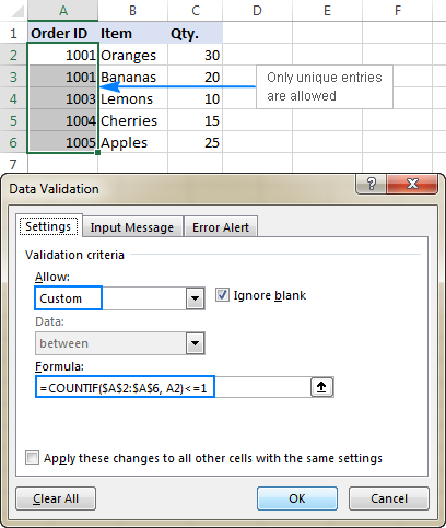
For example, to make sure that only unique order ids are input in cells A2 to A6, create a custom rule with this data validation formula:
=COUNTIF($A$2:$A$6, A2)<=1
When a unique value is entered, the formula returns TRUE and the validation succeeds. If the same value already exists in the specified range (count greater than 1), COUNTIF returns FALSE and the input fails validation.
Please pay attention that we lock the range with absolute cell references (A$2:$A$6) and use a relative reference for the top cell (A2) to get the formula to adjust properly for each cell in the validated range.
Note. This data validation formulas is case-insensitive, it does not distinguish uppercase and lowercase text.
Validation formulas for dates and times
Inbuilt date validation provides quite a lot of predefined criteria to restrict users to entering only dates between the two dates you specify, greater than, less than, or equal to a given date.
If you want more control over data validation in your worksheets, you can replicate the inbuilt functionality with a custom rule or write your own formula that goes beyond the built-in capabilities of Excel data validation.
Allow dates between two dates
To limit the entry to a date within a specified range, you can use either the predefined Date rule with the "between" criteria or make a custom validation rule with this generic formula:
Where:
- cell is the topmost cell in the validated range, and
- start and end dates are valid dates supplied via the DATE function or references to cells containing the dates.
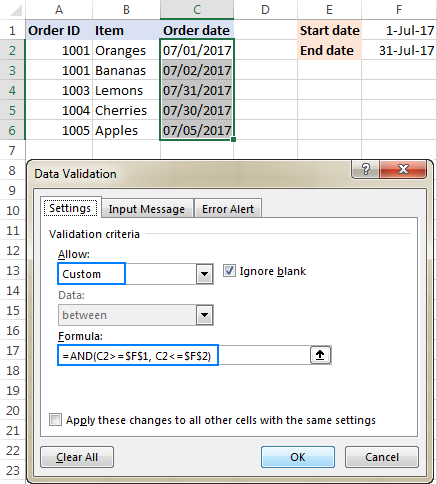
For example, to allow only dates in the month of July of the year 2017, use the following formula:
=AND(C2>=DATE(2017,7,1),C2<=DATE(2017,7,31))
Or, enter the start date and end date in some cells (F1 and F2 in this example), and reference those cells in your formula:
=AND(C2>=$F$1, C2<=$F$2)
Please notice that the boundary dates are locked with absolute cell references.
Allow weekdays or weekends only
To restrict a user to entering only weekdays or weekends, configure a custom validation rule based on the WEEKDAY function.
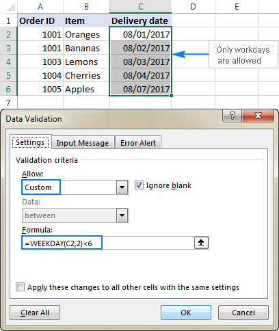
With the return_type argument set to 2, WEEKDAY returns an integer ranging from 1 (Monday) to 7 (Sunday). So, for weekdays (Mon to Fri) the result of the formula should be less than 6, and for weekends (Sat and Sun) greater than 5.
Allow only workdays:
Allow only weekends:
For example, to allow entering only workdays in cells C2:C6, use this formula:
=WEEKDAY(C2,2)<6
Validate dates based on today's date
In many situations, you may want to use today's date as the start date of the allowed date range. To get the current date, use the TODAY function, and then add the desired number of days to it to compute the end date.
For example, to limit the data entry to 6 days from now (7 days including today), we are going to use the built-in Date rule with the formula-based criteria:
- Select Date in the Allow
- Select between in the Data
- In the Start date box, enter
=TODAY() - In the End date box, enter
=TODAY() + 6
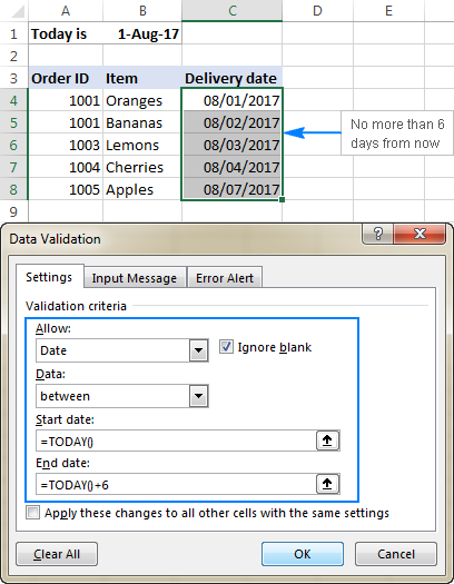
In a similar manner, you can restrict users to entering dates before or after today's date. For this, select either less than or greater than in the Data box, and then enter =TODAY() in the End date or Start date box, respectively.
Validate times based on current time
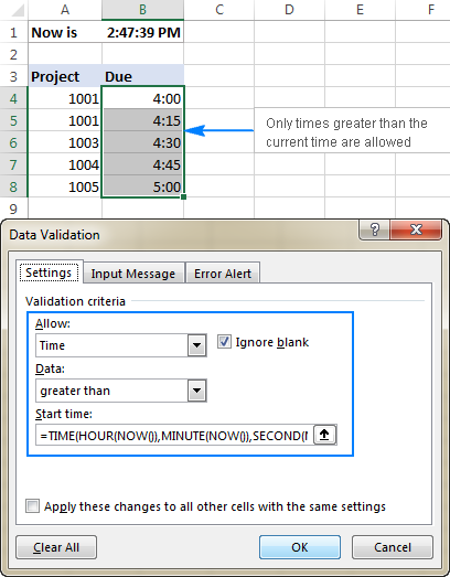
To validate data based on the current time, use the predefined Time rule with your own data validation formula:
- In the Allow box, select Time.
- In the Data box, pick either less than to allow only times before the current time, or greater than to allow times after the current time.
- In the End time or Start time box (depending on which criteria you selected on the previous step), enter one of the following formulas:
- To validate dates and times based on the current date and time:
=NOW() - To validate times based on the current time:
=TIME( HOUR(NOW()), MINUTE(NOW()), SECOND(NOW()))
- To validate dates and times based on the current date and time:
The screenshot below shows a rule that allows only times greater than the current time:
Custom Excel data validation rule not working
If your formula-based data validation rule does not work as expected, there are 3 main points to check:
- Data validation formula is correct
- Validation formula does not refer to an empty cell
- Appropriate cell references are used
Check the correctness of your Excel data validation formula
For starters, copy your validation formula into some cell to make sure it does not return an error such as #N/A, #VALUE or #DIV/0!.
If you are creating a custom rule, the formula should return the logical values of TRUE and FALSE or the values of 1 and 0 equating to them, respectively.
If you use a formula-based criteria in a built-in rule (like we did to validate times based on the current time), it can also return another numeric value.
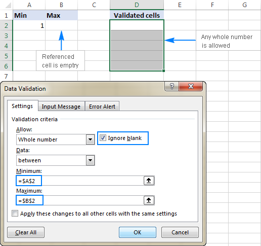
Excel data validation formula should not refer to an empty cell
In many situations, if you select the Ignore blank box when defining the rule (usually selected by default) and one or more cells referenced in your formula is blank, any value will be allowed in the validated cell.
Here is an example in the simplest form:
Absolute and relative cell references in data validation formulas
When setting up a formula-based Excel validation rule, please keep in mind that all cell references in your formula are relative to the upper left cell in the selected range.
If you are creating a rule for more than one cell and your validation criteria are dependent on specific cells, be sure to use absolute cell references (with the $ sign like $A$1), otherwise your rule will work correctly only for the first cell. To better illustrate the point, please consider the following example.
Supposing, you want to restrict data entry in cells D2 to D5 to whole numbers between 1 (minimum value) and the result of dividing A2 by B2. So, you calculate the maximum value with this simple formula =A2/B2, like shown in the screenshot below:
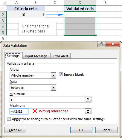
The problem is this seemingly correct formula won't work for cells D3 to D5 because relative references change based on a relative position of rows and columns. Thus, for cell D3 the formula will change to =A3/B3, and for D4 it will become =A4/B4, doing data validation all wrong!
To fix the formula, just type "$" before the column and row references to lock them: =$A$2/$B$2. Or, press F4 to toggle between different reference types.
In situations when you want to validate each cell based on its own criteria, use relative cell references without $ sign to get the formula to adjust for each row or/and column:
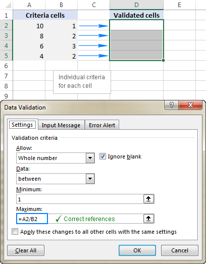
As you see, there is no "absolute truth", the same formula could be right or wrong depending on situation and your particular task.
This is how to use data validation in Excel with your own formulas. T gain more understanding, feel free to download our sample workbook below and examine the rule settings. I thank you for reading and hope to see you on our blog next week!
Practice workbook for download
Excel Data Validation examples (.xlsx file)
 by
by
265 comments
Please I am trying to do a cell validation for text such that if the cell was ignored and left blank, It will display an error message.
I know if you input a text and then delete it, it would display the intended error message. However, I found if you just ignore and skip the cell, no error message is displayed.
How do I resolve this?? Like I do not want any cells omitted or ignored and file can't be closed/saved unless information is complete.
I used the custom, unchecked "ignore blank" and formula : istext()
You can't do this with data validation.
Specifically, you can't prevent the user closing/saving the file half-way through. You could possibly do that with VBA/macro code that is triggered when the file is closed and checks the status of a checkcell.
Without VBA, you could use Conditional Formatting to highlight the empty cells, as well as Data Validation as you describe. That would alert the user to the empty cells, but you can't stop them closing or saving the file.
Thanks Chadwick. I thought as much too that I will probably need VBA to do that.
Hello, I want to restrict the cell with certain alphabet and certain range of numerical value to design a mark ledger of students. I tried to do it but I couldn't. Please, help me.
Hello Amit Kr. Karn
Formula Use in Data Validation Option
there formula
=AND(ISnumber(A1),LEN(A1)=10)
Number Validation 10 digit
there formula text validation 10 text
=AND(IStext(A1),LEN(A1)=10)
i hope you try.
Sorry I completely forgot to escape my angle brackets
A2:-
=IF(B2="",AND(A2>=TIME(0,0,1),A2<=TIME(11,59,59)),AND(A2>=TIME(0,0,1),A2<=B2-TIME(0,0,1)))
B2:-
=IF(A2="",AND(B2>=TIME(0,0,1),B2<=TIME(11,59,59)),AND(B2>=A2+TIME(0,0,1),B2<=TIME(11,59,59)))
Apologies that formula again
=IF(A2="",AND(B2>=TIME(0,0,1),B2=A2+TIME(0,0,1),B2<=TIME(11,59,59)))
Something went wrong with the middle bit.
That second cell formula:-
B2:-
=IF(A2="",AND(B2>=TIME(0,0,1),B2=A2+TIME(0,0,1),B2<=TIME(11,59,59)))
(which actually goes in D2 - to be REFERRED to by B2 . . . )
Hi
Validating 2 neighboring cells (e.g. A2 & B2) to be Start and Finish times SHOULD be done with custom validation formulae . . .
A2:-
=IF(B2="",AND(A2>=TIME(0,0,1),A2=TIME(0,0,1),A2=TIME(0,0,1),B2=A2+TIME(0,0,1),B2<=TIME(11,59,59)))
. . . and these work fine, while the neighbouring cell is NOT BLANK.
When the neighboring cell is BLANK, the validation allows ANY VALUE.
The thing is: there already IS provision for the neighboring cell being blank (it's just that Excel ignores it)
Fortunately, the FULL validation holds - even when the neighboring cell is BLANK - if you put the above formula in e.g. cells C2 and D2 and have the validation formulae REFER to these:-
A2:-
=C2
B2:-
=D2
Hope this helps somebody. I only discovered the problem by accident: you just ASSUME the end user will always enter a time!
HI
I NEED TO PREVENT USER TO ENTER DATA IN WHOLE COLUMN LIKE COL A
EXCEPT IF HE ENTER ANY OF THE FOLLOWING VALUE
( V+D OR D OR V )
Hi Guys
I have an excel drop down list that has options in words for eg low, medium and high as the options. However once an option is selected the cell below the drop down list registers a numeric value for instance low is 1, medium is 2 and high is three. This allows the selection to drive formula in other parts of the sheet and workbook that require numeric input such as the choose formula. Any idea how this is done as am stuck.
Thanks
Hi Ross,
On a separate sheet (not obligatory, but it's neater), create your list. Column A is the numbers 1,2,3, column B is the words.
In the Data Validation dialogue box, set the List to point at the list you just wrote. Just the three cells with the words.
In the cell beneath, where you want a number to appear, enter a vlookup formula. If your Data Validation cell in A1 and the number cell is A2, it would look like this:
=VLOOKUP(A1,Sheet1!$A$1:$B$3,2,FALSE)
Note that in this example, the reference is A1 is dynamic and will change if you copy the formula to other cells. The reference to the list is locked because you don't want that to change.
Alternatively, instead of making a cell with a number and referring to that from your Choose function, you could make the vlookup part of the Choose statement.
Is there any limit of characters to enter a formula in formula bar of Data validation?
I copied a formula from a cell. Then I am creating a data validation for another cell. I am not able to paste the copied formula in the Setting/ allow/ custom/ formula in Data validation? please suggest how to paste a copied formula in formula bar of Data validation?
Formula copy in formula bar not a cell copy dude
Hi
You formula =TIME( HOUR(NOW()), MINUTE(NOW()), SECOND(NOW()))
is not quite correct. There should be > sign
You article is awesome. All other formulas are working
Hi, I need to restrict alphanumberic entry and not more than 200 characters in a cell, together, what formula should I use in the data validation - customer drop down.
Please adivse. Many Thanks
I have a requirement where user should not be allowed to use any excel formula like sum,+J1 for copying the cell value.Basically i want user to should be restricted for using any formal in excel.
Please guide
Hello Supriya,
First go to special option Select formula auto select there formula you put area and use shortcut key Ctrl+1 Tab open Format Cell select tab protection select hidden option and which area not lock select locked option remove than you protection worksheet use password now you can see all password hidden not any copy your formula only show answer.
i hope you will try.
Hi plz help me to solve the validation rule-based ie, not more or less than 100
I am using excel to create a form, one of the cells is for current job title. But in another section I have "New" job title, both the current and new job title are used for calculations. So what I'm trying to do is if there is nothing in the "new" cell it will equal the "current" or if they need to change the title there is a validation drop down list. Right now it seems I can only do one or the other not both. Can you help me?
Hi,
I don't want the user to enter data in a third cell (C1) as the first (A1) and second cells (B1) are empty
I want the user must get a warning message Whenever user trying to enter it on third cell (C1) and it should not show the warning message when (A1) & (B1) are not empty.
Can we do it with data validation?
Thanks,
Hi, I wanted to restrict data entry in a specific format which would be as follows:
dd/mm - dd/mm
This cell will not be in a date format. What I required the user to input date range (as text), for example, 01/11 - 15/11 or 16/12 - 31/12. Is this possible with data validation.
Thanks for your great work.
Good morning. I have a team and each member has their own alpha split and I need to be able to restrict their input into cells depending on the first name of the customers initial.
Basically I need data validation to show an error if a user enters a name not within their split eg one user deals with customers surnames beginning with the initials A to F
I have tried a few variations eg =countif(b3,"a-*")+countif(b3,"b-*") etc but no luck so far.
Any help greatly appreciated. Thanks
Why would a simple validation formula,=(A1+A2) fail, i.e., accepts entries that are not equal to the contents of A1 + A2??
Hi John,
If you select "Custom" in the Allow box, the formula fails indeed. However, if you allow "Whole number" equal to =A1+A2, it works. I cannot say why.
Hi,
I just wanna ask if I can use data validation if i want to restrict the text to be inputted. Example, Middle Name to be inputted but the user input Middle Initial Only. Is it possible to prompt "error" message using data validation? If yes, how? Thanks
I created a list called test1. In this list are part numbers some of these PN's are specific i.e. D2301-00-03 where as other are a range represented with wildcards i.e. 100-N*** which covers a part number range from 100-N000 through 100-999. The length of the part numbers may be different and the placement of letters and numbers may be different as seen above.
I am trying to limit data entry into a cell (A1) only if it matches this list.
I have attempted to do this using the COUNTIF formula in DATA VALIDATION function in cell (A1). It is not working. Any ideas? Thanks.
I'm trying to highlight in red number ranges that is incorrect based on criteria of first cell column for example if Cell A1 has drop down options of NSW,QLD,VIC then in B1 it returns highlights in red cell fill if the number entered in B1 isn't within criteria range for example If Cell A1=NSW then acceptable number range for B1 is 2000-2999 else it highlights the cell in B1 in red and if A1=QLD then B2 should be between 4000-4999 else it highlights that cell in red.
Is this something doable with custom formula?
HOW TO RESTRICT DUPLICATE MOBILE NO IN A SPECIFIC COLUMN
HI LAKSHMI,
USE THIS METHOD
=COUNTIF(A2:C30,A2)=1
Hello,
IN (Excel data validation to allow text only). I want that no one will be able to enter John 1 or John22. Because in this context I can enter John 1 or John 22. But i want that if someone enter john1 by mistake than it will show the Error message.
If I want to create a sheet where if one does not put any data (left it just blank) in one cell, suppose B2, he can't put any data in C2 ... How to do it?
Every code start with unique value and fixed value plzz.. solve the question
Can anyone tell me a quick and easy way of validating the following:
I've got a series of questions with Yes/No validation already set up. However, if No is recorded is B2 and the next 2 questions (C2 and D2) only apply if the answer to B2 is Yes, how do I prevent someone recording a response in C2 and D2 and automatically record a N/A?
Hope that makes sense.
I am trying to format and or validate a cell in Excel 2013 to allow only a certain format. I want a six digit (customer ID) that can only start with a letter (either A, B, D, G or J)) and has exactly 5 digits following the letter. Anyone have any clue how to make this happen?
Rik:
You can use a list for the letters. This can be a drop down box in the entry cell. The five digit numbers can be in an adjacent cell.
Using the letters create a data validation list.
Then select a cell to create the first validation cell.
Select Data tab and choose Validation.
Then in the validation window in the Allow field select the List option and enter the cell range that contains your letters. Be sure to check the in-cell drop down box. Then click OK.
The number validation is the same process except in the Validation window you select Text Length from the Allow field, Equal to from the Data field and type in the number 6 in the Length field.
If you need the data to be in one cell then you can concatenate the cells.
Hi,
I have a requirement where a cell should allow a few specific text entries (OR) Allow decimal values only in a range (ex: -200.00 to 200.00).
Please help me.
Thanks
Hi. Love your work!
Is it possible to have a data validation character limit on a concatenated cell? Example : Cell C1 has formula =A1&B1. I don't want the characters in C1 to exceed 20. I've tried custom data validation with formula =LEN(A1)+LEN(B1)<=20, but it doesn't work. Any suggestions?
Thank you
Kiwi:
I don't think you need to customize the Data Validation in Excel. Just select "Text Length" from the first drop down and then "less than or equal to" in the second field
and enter "20" in the third field. Be sure to check or uncheck the "Ignore Blanks" check box, then enter the message to users in the message tabs and that should work.
Thanks Doug
That's what I tried first. It doesn't work, as it's looking at the text length of the formula, and not the results (I think). =A1&B1 only has 6 characters.
Kiwi:
Each time I've tested that technique it works.
Are there a bunch of spaces or other blank characters in A1 or B1?
Thanks for writing article
Good day.
I am having a strange issue with use of formula while creating a Data validation drop-down list in one of my cells.
Formula =IF(HOVEDTABELL[FAG]="RIE"; RIETEGNINGER;RIBTEGNINGER) is tested and working if entered directly in the main worksheet. true and false conditions route to two different table on neighbouring tabs btw.
When I try to use the same formula while creating a Data validation list, i get the "We found a problem with this formula" warning.
Could you please suggest what could be the issue?
Thank you.
Hey folks,
I need to make few cells required, but in case a user did not do anything on a tab (I have about ten of them in the file) I need to allow a user to save and close the file. Only if a user starts to work at THIS tab I need to force a user to fill in 3 cells within that tab.
Could not find this anywhere, is this doable? All examples I saw invoke a VB scripting and that forces a user to fill in cells unconditionally, simply does not allow to close a file while cells not filed in. Not my case, I have to allow to close a file with these cells empty. And force a user to fill them up only if he/she starts to work at a tab with such condition.
Thanks a lot!
Hi, I want to lock some cells in a form, but would like to do it with validation. Is it possible?
thnaks!
I have the same problem. I tried to make the cell equal itself in the custom formula. That stops the user from changing to another text entry but is allowing numbers. Did this ever get resolved?
validate for text length less than 0, obviously this will never be true, so no input is possible
unless someone copies something there, of course
how do I use data validation (a list or a formula) so that I can restrict the data entry to be only
capital letters
& (the ampersand sign)
, (a comma)
. (a period)
=IF(M2"";ISTEXT(L2),ISNUMBER(L2)) - why not working. If any value is there in m2, the l1 should accept numbers or else text
Hello,
Please try the following formula:
=IF(ISBLANK(M2),IF(ISTEXT(L2),T(L2),TEXT(L2,"@")),VALUE(L2))
Hope it will help you.
what sign is the use in formula for "does not equal too" like
IF(G6="does not equal too either does not blank",VLOOKUP(G6,A6:C19,2,0),"")
Hi Amit,
The "not equal to operator" in Excel is <>
For example:
=IF(AND(G6<>"text", G6<>""),VLOOKUP(G6,A6:C19,2,0),"")
How do I use a validation list and be able to input other data?
Thanks for the instructions! How should a data validation formula look if I'm trying to specify that cells in a particular column should be formatted in either MMDDYEAR or MMDDYEAR ## format? 01, 02, etc. are added to the end of rows with the same date. (ex. 07071980, 07071980 01)
Hello, Lisa,
I can suggest you the following formulas:
1. In case the values are entered in the MMDDYEAR format:
=AND(NOT(ISERROR(DATE(MID(A1,5,4),LEFT(A1,2),MID(A1,3,2)))),VALUE(LEFT(A1,2))<13,VALUE(LEFT(A1,2))<>0,VALUE(MID(A1,3,2))<>0,LEN(A1)=8)
2. In case the values are formatted as MMDDYEAR ##:
=AND(NOT(ISERROR(DATE(MID(A1,5,4),LEFT(A1,2),MID(A1,3,2)))),VALUE(LEFT(A1,2))<13,VALUE(LEFT(A1,2))<>0,VALUE(MID(A1,3,2))<>0,LEN(A1)=11, ISNUMBER(VALUE(RIGHT(A1,2))))
If neither of the formulas above help you, I’m afraid you need to use a special macro then. We do not cover the programming area (VBA-related questions). Please try to find the solution in VBA sections on mrexcel.com or excelforum.com.
Sorry I can't assist you better.
Try use this formula for custom validation which prevent any input which start phrase "XYZ" in Cell A1: =search("xyz",A1,1)=1
Thanks for the article. I was having an issue with this validation formula, =IF(IF(D5"",D5,C5)"F",H5="B",IF(IF(F5"",F5,E5)="B",H5="B",OR(H5="M", H5="B"))) and found your article. I had to remove the check for "Ignore Blanks" and check for blanks myself like this, =IF(IF(D5"",D5,C5)"F",OR(H5="B",TRIM(H5)=""),IF(IF(F5"",F5,E5)="B",or(H5="B",TRIM(H5)=""),OR(H5="M", H5="B",TRIM(H5)=""))) because D5 and F5 did contain blanks making it possible to enter anything even though the formula itself returned a 'False'. You pointed me in the right direction.
What would be the formula on data validation, example the minimum amount is $25 and maximum $300 ?
I've a requirement where i should NOT allow user to enter a value which starts with some phrase like "xyz". Please help me with formula.
Thanks in Advance
I need to create a excel material inventory recording sheet,all material >0 g, must record down the material expiry date.
Example:
If cell A1 is "0", cell A2 must key in "NA"
If ell A1 IS ">0", cell A2 must key in "the expiry date"
I wanted to restrict cell A2 to input date format or "NA" with reference to cell A1, can I use date validate with formula? or any suggestion?
Hello Jayson,
You can use the IF function, e.g. enter the following formula in A2:
=IF(A1=0,"NA","the expiry date")
If you can refer to the expiry date, e.g. if the date is in cell C1, then set the cell format of A2 to date and include the reference:
=IF(A1=0,"NA", C1)
Im having trouble adding to formula i did for custom validation.
The formula points to several lists depending on what is in cell N2.
I have tried this both 'Allow Custom' and 'Allow List' and receive the error:
"There's a problem with this formula.
Not trying to type a formula?
When the first character is an equal(=) . . . "
Not sure why i can update the formula by adding another list reference.
Any ideas?
Thanks
Tam
Hello Tam,
Could you specify what formula you use and what result you need to get? If possible, please send a sample file to support@ablebits.com along with a link to this post and your comment. We'll do our best to assist you.
I created an excel workbook with multiple sheet that does some accounting and mathematics calculation.
Pls how can I turn this workbook to a desktop or mobile application that runs on it own?.
Or which programming language do I have to learn to create an app that calculates using same kind of function in Excel.
Thanks in anticipation.
Hello, Patrick,
I'm sorry but you'd better ask these questions on Mr. Excel forum. They deal with some programming/VBA stuff there, so they may be able to assist you better.
Conditional Formatting Duplicate value does not working when "/" or space is inserted please guide me
example
Khalid Khalid/Asif
Math Bio/Com
I need to convert -ve time value to +ve need your support.
For Example:
-2:20 to 2:20
-1:18 to 1:18
-0:17 to 0:17
Hi Svetlana,
A very short message. You are brilliant, Thank-you
I recently set up the following function in Excel, to look for a list of words in ONE cell, and if it finds any of the words listed in my formula, then 'red-flag' to say "Keyword Exclusion". Again, currently it's looking at only ONE cell (cell 'I2' in the formula below); and it's working beautifully!
However, I now need for the formula to look at a SECOND cell as well. If it finds any of the same words listed in that second cell, then simply perform the same 'red-flag' coding. I've tried different variations of "IF(OR and AND" formulas, but it's not working.
My current formula is as follows:
=IF(SUMPRODUCT(--ISNUMBER(SEARCH({"motor vehicle","construction","public transportation","health","family","criminal","revitalization"},I2)))>0,"Keyword Exclusion","")
Hi Ignacio,
If you want the OR logic, i.e. if any of the words is found either in I2 or, say K2, simply concatenate the two cells like this:
=IF(SUMPRODUCT(--ISNUMBER(SEARCH({"motor vehicle","construction","public transportation","health","family","criminal","revitalization"}, I2&K2)))>0, "Keyword Exclusion","")
If you want the AND logic, i.e. if any of the words is found both in I2 and K2, then check each cell individually:
=IF(SUMPRODUCT(--ISNUMBER(SEARCH({"motor vehicle","construction","public transportation","health","family","criminal","revitalization"},I2)), --ISNUMBER(SEARCH({"motor vehicle","construction","public transportation","health","family","criminal","revitalization"},K2)))>0, "Keyword Exclusion","")
Can you clarify the find and search formulas in the article are correct?
Case-insensitive: =ISNUMBER(SEARCH($A$2:$A$6, A2))
Case-sensitive: =ISNUMBER(FIND($A$2:$A$6, A2))
Based on the rest of the section, should the data range listed be replaced with "AA"? Otherwise, I don't follow how the range helps with SEARCH or FIND.
These articles are great. I always find new ways to improve my sheets.
Hi!
The correct formulas are =ISNUMBER(SEARCH("AA", A2)) and =ISNUMBER(FIND("AA", A2)) as shown in the screenshot. Don't know where those ranges came from. Sorry for the confusion and thank you - the formulas are fixed.
Hi
Using data validation, I know it is possible to do the below separately:
1. Create a data validation drop down list (ALT + A + V + V then select list from the 'Allow' field and denote the cell range in the 'Source' field)
2. Prevent users from entering data into one cell (e.g. cell A2) if another cell (e.g. cell A1) has not yet been populated (ALT + A + V + V then select Custom from the 'Allow' field and insert '=NOT(ISBLANK(A1))' in the 'Formula' field)
However, I am in need of a combination of both. I need to customise a cell such that if cell A1 is not populated, then cell A2 cannot be populated but, when cell A1 has data inserted, A2 should be able to be populated but only through a drop-down list. May you assist