The tutorial explains how to use Excel functions to convert text to date and number to date, and how to turn text strings into dates in a non-formula way. You will also learn how to quickly change a number to date format.
Since Excel is not the only application you work with, sometimes you'll find yourself working with dates imported in an Excel worksheet from a .csv file or another external source. When that happens, chances are the dates will export as text entries. Even though they look like dates, Excel won't not recognize them as such.
There are many ways to convert text to date in Excel and this tutorial aims to cover them all, so that you can choose a text-to-date conversion technique most suitable for your data format and your preference for a formula or non-formula way.
How to distinguish normal Excel dates from "text dates"
When importing data into Excel, there is often a problem with date formatting. The imported entries may look like normal Excel dates to you, but they don't behave like dates. Microsoft Excel treats such entries as text, meaning you cannot sort your table by date properly, nor can you use those "text dates" in formulas, PivotTables, charts or any other Excel tool that recognizes dates.
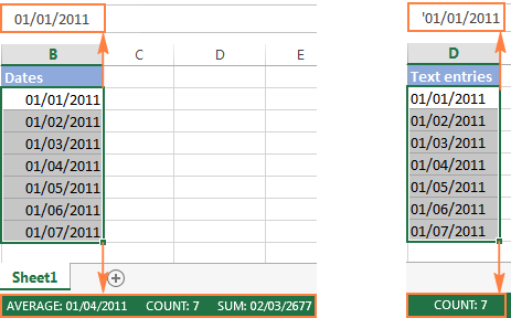
There are a few signs that can help you determine whether a given entry is a date or a text value.
| Dates | Text values |
|
|
How to convert number to date in Excel
Since all Excel functions that change text to date return a number as a result, let's have a closer look at converting numbers to dates first.
As you probably know, Excel stores dates and times as serial numbers and it is only a cell's formatting that forces a number to be displayed as a date. For example, 1-Jan-1900 is stored as number 1, 2-Jan-1900 is stored as 2, and 1-Jan-2015 is stored as 42005. For more information on how Excel stores dates and times, please see Excel date format.
When calculating dates in Excel, the result returned by different date functions is often a serial number representing a date. For example, if =TODAY()+7 returns a number like 44286 instead of the date that is 7 days after today, that does not mean the formula is wrong. Simply, the cell format is set to General or Text while it should be Date.
To convert such serial number to date, all you have to do is change the cell number format. For this, simply pick Date in the Number Format box on the Home tab.
To apply a format other than default, then select the cells with serial numbers and press Ctrl+1 to open the Format Cells dialog. On the Number tab, choose Date, select the desired date format under Type and click OK.
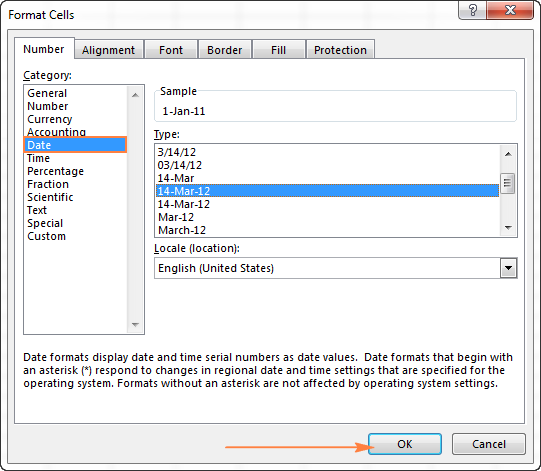
Yep, it's that easy! If you want something more sophisticated than predefined Excel date formats, please see how to create a custom date format in Excel.
If some stubborn number refuses to change to a date, check out Excel date format not working - troubleshooting tips.
How to convert 8-digit number to date in Excel
It's a very common situation when a date is input as an 8-digit number like 10032016, and you need to convert it into a date value that Excel can recognize (10/03/2016). In this case, simply changing the cell format to Date won't work - you will get ########## as the result.
To convert such a number to date, you will have to use the DATE function in combination with RIGHT, LEFT and MID functions. Unfortunately, it is not possible to make a universal formula that will work in all scenarios because the original number can be input in a variety of different formats. For example:
| Number | Format | Date |
| 10032016 | ddmmyyyy | 10-Mar-2016 |
| 20160310 | yyyymmdd | |
| 20161003 | yyyyddmm |
Anyway, I will try to explain the general approach to converting such numbers to dates and provide a few formula examples.
For starters, remember the order of the Excel Date function arguments:
So, what you need to do is extract a year, month and date from the original number and supply them as the corresponding arguments to the Date function.
For example, let's see how you can convert number 10032016 (stored in cell A1) to date 3/10/2016.
- Extract the year. It's the last 4 digits, so we use the RIGHT function to pick the last 4 characters: RIGHT(A1, 4).
- Extract the month. It's the 3rd and 4th digits, so we employ the MID function to get them MID(A1, 3, 2). Where 3 (second argument) is the start number, and 2 (third argument) is the number of characters to extract.
- Extract the day. It's the first 2 digits, so we have the LEFT function to return the first 2 characters: LEFT(A2,2).
Finally, embed the above ingredients into the Date function, and you get a formula to convert number to date in Excel:
=DATE(RIGHT(A1,4), MID(A1,3,2), LEFT(A1,2))
The following screenshot demonstrates this and a couple more formulas in action:

Please pay attention to the last formula in the above screenshot (row 6). The original number-date (161003) contains only 2 chars representing a year (16). So, to get the year of 2016, we concatenate 20 and 16 using the following formula: 20&LEFT(A6,2). If you don't do this, the Date function will return 1916 by default, which is a bit weird as if Microsoft still lived in the 20th century :)
Note. The formulas demonstrated in this example work correctly as long as all numbers you want to convert to dates follow the same pattern.
How to convert text to date in Excel
When you spot text dates in your Excel file, most likely you would want to convert those text strings to normal Excel dates so that you can refer to them in your formulas to perform various calculations. And as is often the case in Excel, there are a few ways to tackle the task.
Excel DATEVALUE function - change text to date
The DATEVALUE function in Excel converts a date in the text format to a serial number that Excel recognizes as a date.
The syntax of Excel's DATEVALUE is very straightforward:
So, the formula to convert a text value to date is as simple as =DATEVALUE(A1), where A1 is a cell with a date stored as a text string.
Because the Excel DATEVALUE function converts a text date to a serial number, you will have to make that number look like a date by applying the Date format to it, as we discussed a moment ago.
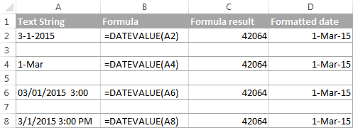
The following screenshots demonstrates a few Excel DATEVALUE formulas in action:
Excel DATEVALUE function - things to remember
When converting a text string to a date using the DATEVALUE function, please keep in mind that:
- Time information in text strings is ignored, as you can see in rows 6 and 8 above. To convert text values containing both dates and times, use the VALUE function.
- If the year is omitted in a text date, Excel's DATEVALUE will pick the current year from your computer's system clock, as demonstrated in row 4 above.
- Since Microsoft Excel stores dates since January 1, 1900 , the use of the Excel DATEVALUE function on earlier dates will result in the #VALUE! error.
- The DATEVALUE function cannot convert a numeric value to date, nor can it process a text string that looks like a number, for that you will need to use the Excel VALUE function, and this is exactly what we are going to discuss next.
Excel VALUE function - convert a text string to date
Compared to DATEVALUE, the Excel VALUE function is more versatile. It can convert any text string that looks like a date or number into a number, which you can easily change to a date format of your choosing.
The syntax of the VALUE function is as follows:
Where text is a text string or reference to a cell containing the text you want to convert to number.
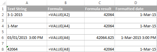
The Excel VALUE function can process both date and time, the latter is converted to a decimal portion, as you can see in row 6 in the following screenshot:
Mathematical operations to convert text to dates
Apart from using specific Excel functions such as VALUE and DATEVALUE, you can perform a simple mathematical operation to force Excel to do a text-to-date conversion for you. The required condition is that an operation should not change the date's value (serial number). Sounds a bit tricky? The following examples will make things easy!
Assuming that your text date is in cell A1, you can use any of the following formulas, and then apply the Date format to the cell:
- Addition:
=A1 + 0 - Multiplication:
=A1 * 1 - Division:
=A1 / 1 - Double negation:
=--A1
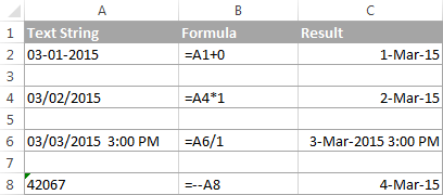
As you can see in the above screenshot, mathematical operations can convert dates (rows 2 and 4), times (row 6) as well as numbers formatted as text (row 8). Sometimes the result is even displayed as a date automatically, and you don't have to bother about changing the cell format.
How to convert text strings with custom delimiters to dates
If your text dates contain some delimiter other than a forward slash (/) or dash (-), Excel functions won't be able to recognize them as dates and return the #VALUE! error.
To fix this, you can run Excel's Find and Replace tool to replace your delimiter with a slash (/), all in one go:
- Select all the text strings you want to convert to dates.
- Press Ctrl+H to open the Find and Replace dialog box.
- Enter your custom separator (a dot in this example) in the Find what field, and a slash in the Replace with
- Click the Replace All
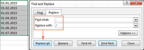
Now, the DATEVALUE or VALUE function should have no problem with converting the text strings to dates. In the same manner, you can fix dates containing any other delimiter, e.g. a space or a backward slash.
If you prefer a formula solution, you can use Excel's SUBSTITUTE function instead of Replace All to switch your delimiters to slashes.
Assuming the text strings are in column A, a SUBSTITUTE formula may look as follows:
=SUBSTITUTE(A1, ".", "/")
Where A1 is a text date and "." is the delimiter your strings are separated with.
Now, let's embed this SUBSTITUTE function into the VALUE formula:
=VALUE(SUBSTITUTE(A1, ".", "/"))
And have the text strings converted to dates, all with a single formula.
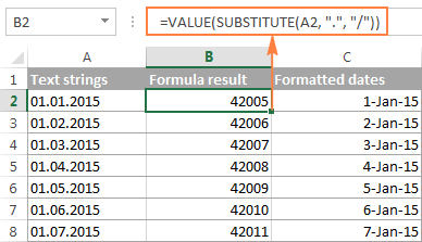
As you see, the Excel DATEVALUE and VALUE functions are quite powerful, but both have their limits. For example, if you are trying to convert complex text strings like Thursday, January 01, 2015, neither function could help. Luckily, there is a non-formula solution that can handle this task and the next section explains the detailed steps.
Text to Columns wizard - formula-free way to covert text to date
If you are a non-formula user type, a long-standing Excel feature called Text To Columns will come in handy. It can cope with simple text dates demonstrated in Example 1 as well as multi-part text strings shown in Example 2.
Example 1. Converting simple text strings to dates
If the text strings you want to convert to dates look like any of the following:
- 1.1.2015
- 1.2015
- 01 01 2015
- 2015/1/1
You don't really need formulas, nor exporting or importing anything. All it takes is 5 quick steps.
In this example, we will be converting text strings like 01 01 2015 (day, month and year are separated with spaces) to dates.
- In your Excel worksheet, select a column of text entries you want to convert to dates.
- Switch to the Data tab, Data Tools group, and click Text to Columns.

- In step 1 of the Convert Text to Columns Wizard, select Delimited and click Next.
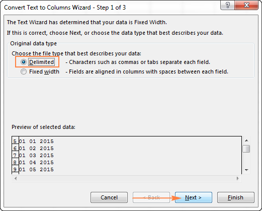
- In step 2 of the wizard, uncheck all delimiter boxes and click Next.
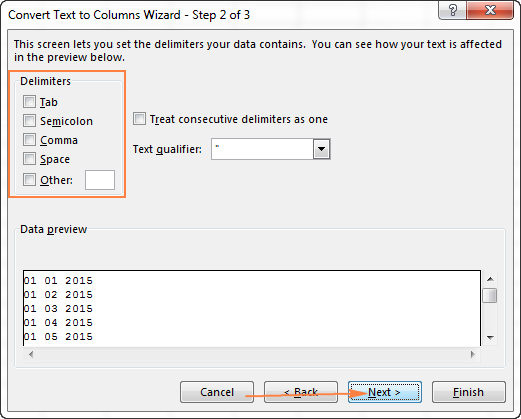
- In the final step, select Date under Column data format, choose the format corresponding to your dates, and click Finish.
In this example, we are converting the text dates formatted as "01 02 2015" (month day year), so we select MDY from the drop down box.
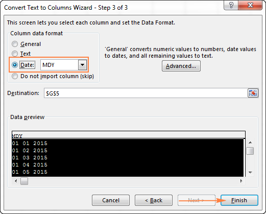
Now, Excel recognizes your text strings as dates, automatically converts them to your default date format and displays right-aligned in the cells. You can change the date format in the usual way via the Format Cells dialog.
Note. For the Text to Column wizard to work correctly, all of your text strings should be formatted identically. For example, if some of your entries are formatted like day/month/year format while others are month/day/year, you would get incorrect results.
Example 2. Converting complex text strings to dates
If your dates are represented by multi-part text strings, such as:
- Thursday, January 01, 2015
- January 01, 2015 3 PM
You will have to put a bit more effort and use both the Text to Columns wizard and Excel DATE function.
- Select all text strings to be converted to dates.
- Click the Text to Columns button on the Data tab, Data Tools group.
- On step 1 of the Convert Text to Columns Wizard, select Delimited and click Next.
- On step 2 of the wizard, select the delimiters your text strings contain.
For example, if you are converting strings separated by commas and spaces, like "Thursday, January 01, 2015", you should choose both delimiters - Comma and Space.
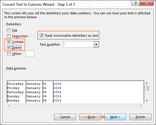
It also makes sense to select the "Treat consecutive delimiters as one" option to ignore extra spaces, if your data has any.
And finally, have a look at the Data preview window and verify if the text strings are split to columns correctly, then click Next.
- On step 3 of the wizard, make sure all columns in the Data Preview section have the General format. If they don't, click on a column and select General under the Column data format options.
Note. Do not choose the Date format for any column because each column contains only one component, so Excel won't be able to understand this is a date.
If you don't need some column, click on it and select Do not import column (skip).
If you don't want to overwrite the original data, specify where the columns should be inserted - enter the address for the top left cell in the Destination field.
When done, click the Finish button.
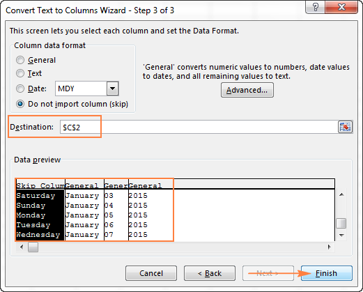
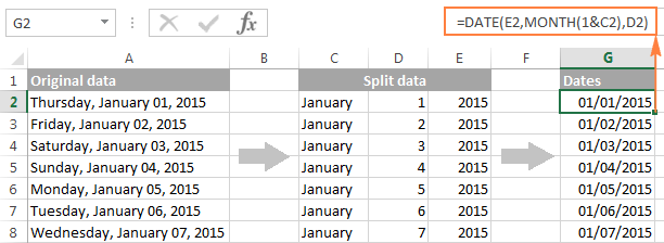
As you see in the screenshot above, we are skipping the first column with the days of the week, splitting the other data into 3 columns (in the General format) and inserting these columns beginning from cell C2.
The following screenshot shows the result, with the original data in column A and the split data in columns C, D and E.

- Finally, you have to combine the date parts together by using a DATE formula. The syntax of the Excel DATE function is self-explanatory:
DATE(year, month, day)
In our case,
yearis in column E anddayis in column D, no problem with these.It's not so easy with
monthbecause it is text while the DATE function needs a number. Luckily, Microsoft Excel provides a special MONTH function that can change a month's name to a month's number:=MONTH(serial_number)For the MONTH function to understand it deals with a date, we put it like this:
=MONTH(1&C2)Where C2 contains the name of the month, January in our case. "1&" is added to concatenate a date (1 January) so that the MONTH function can convert it to the corresponding month number.
And now, let's embed the MONTH function into the
month; argument of our DATE formula:=DATE(F2,MONTH(1&D2),E2)
And voila, our complex text strings are successfully converted to dates:
Quick conversion of text dates using Paste Special
To quickly convert a range of simple text strings to dates, you can use the following trick.
- Copy any empty cell (select it and press Ctrl + C).
- Select the range with text values you want to convert to dates.
- Right-click the selection, click Paste Special, and select Add in the Paste Special dialog box:

- Click OK to complete the conversion and close the dialog.
What you have just done is tell Excel to add a zero (empty cell) to your text dates. To be able to do this, Excel converts a text string to a number, and since adding a zero does not change the value, you get exactly what you wanted - the date's serial number. As usual, you change a number to the date format by using the Format Cells dialog.
To learn more about the Paste Special feature, please see How to use Paste Special in Excel.
Fixing text dates with two-digit years
The modern versions of Microsoft Excel are smart enough to spot some obvious errors in your data, or better say, what Excel considers an error. When this happens, you will see an error indicator (a small green triangle) in the upper-left corner of the cell and when you select the cell, an exclamation mark appears:
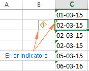
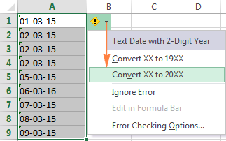
Clicking the exclamation mark will display a few options relevant to your data. In case of a 2-digit year, Excel will ask if you want to convert it to 19XX or 20XX.
If you have multiple entries of this type, you can fix them all in one fell swoop - select all the cells with errors, then click on the exclamation mark and select the appropriate option.
How to turn on Error Checking in Excel
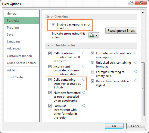
Usually, Error Checking is enabled in Excel by default. To make sure, click File > Options > Formulas, scroll down to the Error Checking section and verify if the following options are checked:
- Enable background error checking under Error Checking;
- Cells containing years represented as 2 digits under Error checking rules.
How to change text to date in Excel an easy way
As you see, converting text to date in Excel is far from being a trivial one-click operation. If you are confused by all different use cases and formulas, let me show you a quick and straightforward way.
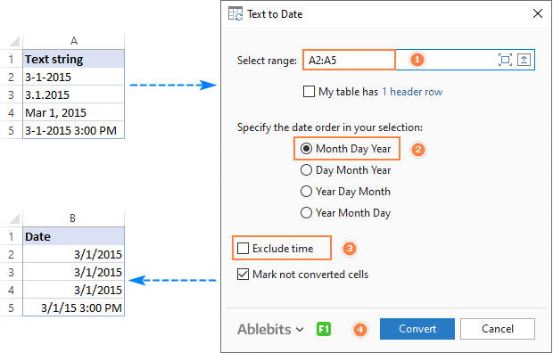
Install our Ultimate Suite (a free trial version can be downloaded here), switch to the Ablebits Tools tab (2 new tabs containing 70+ awesome tools will be added to your Excel!) and find the Text to Date button:

To convert text-dates to normal dates, here's what you do:
- Select the cells with text strings and click the Text to Date button.
- Specify the date order (days, months and years) in the selected cells.
- Choose whether to include or not include time in the converted dates.
- Click Convert.
That's it! The results of conversion will appear in the adjacent column, your source data will be preserved. If something goes wrong, you can simply delete the results and try again with a different date order.
Tip. If you chose to convert times as well as dates, but the time units are missing in the results, be sure to apply a number format that shows both the date and time values. For more info, please see How to create custom date and time formats.
If you are curious to learn more about this wonderful tool, please check out its home page: Text to Date for Excel.
This is how you convert text to date in Excel and change dates to text. Hopefully, you have been able to find a technique to your liking. In the next article, we will tackle the opposite task and explore different ways of converting Excel dates to text strings. I thank you for reading and hope to see you next week.
 by
by
710 comments
Thanks a lot.
Hello Alexander,
First of all, great work here helping everybody out! Thanks for that.
My question is a bit different from most. I have dates like this: early Jan 2021, middle Jan 2021 and late Jan 2021 for example.
From this info a new date should appear in the next column.
- Early Jan 2021 > 25-02-2021
- Middle Jan 2021 > 05-03-2021
- Late Jan 2021 > 15-03-2021
I can turn Early Jan 2021 into dates by using the replace function to turn the word Early into 05.
My question is how do I go from 05 Jan 2021 in one cell to 25-02-2021 in another?
I hope I made myself clear.
Thanks again!
Hello!
If I understand your task correctly, the following formula should work for you:
=DATEVALUE(SUBSTITUTE(A1,"Early",5,1))+51
I hope this will help, otherwise please do not hesitate to contact me anytime.
I'm sorry, I don't quite understand what's happening in this formula.
What should be in cell A1 in this example? And what would be the output of this formula?
Hi,
In A1, write "Early Jan 2021". You will receive the date 25-02-2020
I think my Excel might be different. The variables for my SUBSTITUTE function are: (text; old_text; new_text; [instance_num])
Ah! If I delete the instance number it works! Thank you so much.
Thank you for your help Alexander and it works, but only for January. If I use February for example it does not return 25-03-2021 but instead 28-03-2021. I guess what I am trying is a bit too complicated.
Also would there be a way to make the formula conditional? So Early would be changed to 5, Middle would be changed to 15 and Late would be changed to 25?
Hello!
I wrote this formula based on the description you provided in your original comment. Please note that if you’d provided me with the precise and detailed description of your task from the very beginning, I’d have created a different formula that would have worked for your case.
=IF(ISNUMBER(SEARCH("early",A1,1)), EDATE(DATEVALUE("1 "&MID(A1,FIND(" ",A1,1)+1,50)),1)+24,
IF(ISNUMBER(SEARCH("middle",A1,1)), EOMONTH(EDATE(DATEVALUE("1 "&MID(A1,FIND(" ",A1,1)+1,50)),1),0)+5,
IF(ISNUMBER(SEARCH("late",A1,1)), EOMONTH(EDATE(DATEVALUE("1 "&MID(A1,FIND(" ",A1,1)+1,50)),1),0)+15,"")))
I'm having a hard time with this:
C2 has a custom date format of 2020-10-21 and is set using custom formatting built into Excel
D2 has a static general formatted number of lets say 0085001832000
E2 has a digit, lets use 9
F2 has a custom formatted "date" that was added to the custom formatting selection of yymmdd and is pulling from the date from C2 in a yyyy-mm-dd custom format (i.e. 201021).
G2 has a number in a text format of 20200045
My issue is when I try to combine D2, E2, F2 and G2 into H2, everything works out great with the exception of the Date from cell F2. The combined string says 00850018320009"1144124"20200045. I'm not sure what's happening with the area in "" which should be the date information in F2. Anyone have any idea why it's converting it into what appears to be a number that represents the date?
Hello!
Dates are stored in Excel as numbers. If you want to add a date to a text string, then you need to convert the date to text with TEXT function. Read more in this guide.
If there is anything else I can help you with, please let me know.
I managed to convert some dates as MMDDYYYY to MM-YR. However, only half converted. The rest remains as MMDDYYYY. How do I format the balance?
Hello!
Unfortunately, without seeing your data it is difficult to give you any advice. Please provide me with an example of the source data and the expected result. I can assume that some dates are written as text. What does format mean MM-YR ??
It means Month-Year
If you do not explain how I asked, I cannot help you.
In A2 column I have 200 hundreds of dates as a text string, like, how to get all these into MMDDYYYY format? Here I only know with an open eye which one is a year, and the month and days are confusing.
1949/5/2
2-3-2002
09/11/1988
11/12/1987
03/02/1999
02-08-91
Hello!
All of your dates are spelled differently. Therefore, you need to write a formula for each of them. Use the guidelines in this article, as well as the DATE, LEFT, MID, RIGHT functions.
You will find many ways to convert text to date in the comments to this article.
Hello,
I have a transaction date and time as text, 2020092120371600. I need it to display as date and time, including the seconds, in a single cell. Ideally the above would display as 09/21/20 21:37 16:00, where the 16:00 represent seconds. Can this be done such that the column of transactions date/times can be sortable? Thanks in advance for assistance with this.
Hello!
To convert your text to date and time, use the formula
=DATE(LEFT(A1,4),MID(A1,5,2),MID(A1,7,2))+TIME(MID(A1,9,2),MID(A1,11,2),MID(A1,13,2))
Use a custom date and time format too
mm/d/yyyy hh:mm SS:"00"
I hope my advice will help you solve your task.
This worked perfectly! Thank you!
In certain cases, the last 2 digits in my time stamp are not "00". Maybe this is called hundredths of a second? Can Excel also handle this via formatting? Even though the value is very, very small, it does make a difference in my sort-order. An example would be; 2020091712225895
Hello!
Change the formula to show milliseconds
=DATE(LEFT(D1,4),MID(D1,5,2),MID(D1,7,2)) + TIME(MID(D1,9,2),MID(D1,11,2), MID(D1,13,2)) + (1/24)/60/60/1000*RIGHT(D1,2)
Milliseconds are usually 3 digits. If you only use 2 digits then
=DATE(LEFT(D1,4),MID(D1,5,2),MID(D1,7,2)) + TIME(MID(D1,9,2),MID(D1,11,2), MID(D1,13,2)) + (1/24)/60/60/1000*RIGHT(D1,2)*10
Also use another custom date and time format
mm/d/yyyy hh:mm ss.000
Every last decimal and digit looks great? I really am thankful for your time to help with this. I know how you did this, but I struggle writing these. It's like magic when I double-click the cross that populates the column on down. Cheers!
i am very thankful to you if you convert text
Jan 15, 2021 15:33:25
in to 15,1,2021 and 15:33:25
I solved it myself! :3
I hope is useful for someone else.
Sep 7 2020 5:14PM
Sep 11 2020 1:12AM
Sep 18 2020 10:18PM
Mar 3 2020 10:34PM
first column
=date(MID(A2,8,4),MONTH(1&LEFT(A2,3)),MID(A2,5,2))
second column
=TIMEVALUE(MID(A2,13,5)&" "&RIGHT(A2,2))
Regards.
Need to convert the following format into two columns. So it will look like this:
Sep 7 2020 5:14PM 09/07/2020 5:14 PM
Sep 11 2020 1:12AM 09/11/2020 1:12 AM
Mar 3 2020 10:00PM 03/03/2020 10:00 PM
Thank you for your support.
To make it a little bit more clear. Type A to Type B:
Type A
Mar 3 2020 10:00PM (:00PM is not a typo, that's how the system gives me the value)
TYPE B
COLUMN 1----COLUMN2
03/03/2020---- 10:00 PM
Hello!
If I understood correctly, you want to split the text into 2 parts. Use "M" as separator.
Please use the following formula:
=LEFT(A1,FIND("M ",A1,1))
=RIGHT(A1,LEN(A1)-FIND("M ",A1,1)-1)
Hello Alexander!
I'm sorry but that's not what I want to do. On COLUMN A it will show the text "Mar 3 2020 10:34PM"
What I want is that in COLUMN B will show the date in number format>>> 03/03/2020
And in COLUMN C it will show the time>>> 10:34 PM
I tried the formulas that you provided and they gave me #VALUE! error.
The CSV text comes like this:
Sep 7 2020 5:14PM
Sep 11 2020 1:12AM
Sep 18 2020 10:18PM
Mar 3 2020 10:34PM
I want to make it: mm/dd/yyyy
And on another column: h:mm AM/PM
Hello!
The formula I sent to you was created based on the description you provided in your first request. However, as far as I can see from your second comment, your task is now different from the original one. Hence, the formula fails to work.
Dear sirs, can I ask for a wee bit of your expertise since my own is not enough in this case?
I am looking to do comparisons between quarters during the year but with the closing balance date fixed from previous year. Let me explain:
E.g. QUARTER 4(b)=2020-12-31, QUARTER 3(c)=2020-09-30, Closing balance (QUARTER 4(a))=2019-12-31.
I have created formulas for Q4(b) and Q3(c) (linked to another date cell) respecively so that when Q4(b)=>Q1(b), Q3(c)=>Q4(c). But, i want the Closing balance date Q4(a) (ie. 2019-12-31) to remain the same during the year UNTILL the new accounting year starts. So when Q1(b)=2021-03-31, Q4(c)=2020-12-31 and Q4(a)=2020-12-31.
In words, Q(b) and Q(c) change during the year where Q(a) remain the same with previous year's closing date, and it's only when the Q(b)/Q(c) year change as Q(a) changes closing date one year forward.
I find the Q(a) value quite tricky to solve.
Thank you and regards,
Daniel
I cannot do calculation with "9/25/2019 12:00:00 AM". It seems it is text. How can I convert it to "Sep 25 2019"? I want to do a subtraction with another cell in that format to get the days in between.
Hello!
If your date is written as text, you can convert it to a real date using the formula
=DATE(MID(E1,FIND("~",SUBSTITUTE(E1,"/","~",2),1)+1,FIND(" ",E1,1) - FIND("~",SUBSTITUTE(E1,"/","~",2),1)-1), LEFT(E1, SEARCH("/",E1,1)-1), MID(E1,FIND("~",SUBSTITUTE(E1,"/","~",1),1)+1, FIND("~",SUBSTITUTE(E1,"/","~",2),1) - FIND("~",SUBSTITUTE(E1,"/","~",1),1)-1))
Then set the date format you want in the cell.
How do I covert this number to a date - Month/Day/Year
I tried this formula and it does not work.
=DATE(RIGHT(A2,4), MID(A2,3,2), LEFT(A21,2)) 1/6/2020
Posting Date Transaction Date
06012020 05292020
06012020 05282020
06012020 05292020
Hello!
The formula
=DATE(RIGHT(A2,4), MID(A2,3,2), LEFT(A2,2))
or
= MID(A2,3,2)&"/"&LEFT(A2,2)&"/"& RIGHT(A2,4)
works.
I have imported data from our school information system. Birthdays are showing as 8/20/2002. I need the format to be a text before I can upload the file to another system. The format has to be in mmddyyyy, which I have done so my cell now shows 08202002, but I need it to be recognized as text, not a date before I upload it. If I try to convert it to text, it shows the number 37498, which I understand is the number of days since Jan. 1 1900. How do I get the cell to recognize 08202002 as text and no longer as a date? If I upload it as it is showing, I receive an error stating my date is in the wrong format, because it is still showing as a date not a number.
Thank you.
Hello!
If I understand your task correctly, the following formula should work for you:
=TEXT(F10,"mmddyyyy")
How to convert date to text read more here.
Hi Alexander
Please help to convert
8/19/2020 7:37:23 PM in General to 19-08-2020 19:37
Hello!
If your data is written as text, use the DATEVALUE function. Please read the above article carefully.
HI ,
I HAVE TRIED DATEVALUE BUT NOT NOT WORKED.Please help to take a difference for two entries as they are text strings.Thanks
8/14/2020 7:48:53 AM 8/17/2020 12:29:35 PM
Hello!
What is the date format on your computer - dd/mm/yyyy or mm/dd/yyyy? If the format is mm/dd/yyyy, then your text should be automatically converted to date.
Thank you so much for this! This is very helpful!
Hello
How do i please convert this "40464% order date in cell C2 into a normal date format
Hi. Previously, if I type "8-10" it would be treated as mmdd resulting to "Aug-10" or depending on default format. Now, excel treats "8-10" as ddmm and shows October-08. Is there a way to change the default syntax of typing dates without having to change the date format every new excel worksheet?
Hello,
How to convert 2020-04-17T10:58:58Z to DD/MM/YYYY
Thank You
Hello!
If I understand your task correctly, the following formula should work for you:
=DATE(--LEFT(D3,4),--MID(D3,6,2),--MID(D3,9,2))
The formula returns the date. You can use any date format you need.
Hi!
I have a question, I wanted to get a continuous string of yyyymmm, but if I do it I get something like 201913. For example, I started off with date 201906, and I wanted that to keep going into 202006 without me having to change the 201913, 201914, 201915 etc. Is there a way to do this? For my formula I just do the cell+ 1, which is why i get the 201913.
Thank you!
Hello!
If you wanted the string "yyyymmm" then 201913 is not possible. After all, month 13 does not exist! So what numbers do you want? In addition, if you add 1 to the date, it means +1 day, not +1 month.
Hello, I want to put 3 reminder dates at least in one cell, and then used those dates to determine the last activity date of all dates in my sheet, meaning there would be different cells selected which will have one single date. Formating for reminder dates would be (01/06/2020 (alt+enter) 06/06/2020 (alt+enter) 12/06/2020)
Hello!
In this case, your dates will be written as text. Explain what you want to do with these cells? Give an example of the desired result. It’ll help me understand it better and find a solution for you. Thank you.
Hi Alexander,
I need to convert YYYYMMDD to MMDDYY for all the cells is it possible. Please help
Hello Shruthi!
I’m sorry but your task is not entirely clear to me. Could you please describe it in more detail? Is your data recorded as a date or as text? Do you want to get the result as a date or as text? Write an example of the source data and the result you want to get.
Hi,
I need to convert dates in the following format - MMYY - from TEXT to DATE format. The dates are entered as follows:
114 for 01/1/2014
1015 for 10/1/2015
616 for 06/1/2016
The day is always understood to be 1 so it is never entered. The year is always understood to start with 20 so it is never entered. Zeros are never entered in front of single-digit months.
Do you have a formula to convert?
Any help would be appreciated!
Hello Sandra!
To convert text to date, use the LEFT and RIGHT functions
=DATE("20"&RIGHT(A1,2),LEFT(A1,LEN(A1)-2),1)
I hope it’ll be helpful.
I have two columns with date and time stamp as strings ex. June-23-2020 12:38:42 PM.
First I want to convert these to normal date and time format so that I can find time different between two columns. Please suggest.
Hello!
To select a date from your text, use the formula
=DATEVALUE(MID(Z1,FIND(" ",Z1,1)-4,4)&"-" &MATCH(LEFT(Z1,3),{"Jan","Feb","Mar","Apr","May","Jun","Jul","Aug","Sep","Oct","Nov","Dec"}) &"-"&MID(Z1,FIND(" ",Z1,1)-7,2))
To select time from the text, use the formula
=TIMEVALUE(RIGHT(Z1,LEN(Z1)-FIND(" ",Z1,1)))
Hope this is what you need.
I took out an output from some tool which gave me the numeric value of the datetime -
June 25, 2020 16:06:37 as 1593065197208, when i exported it in csv.
i am not sure what 1593065197208 is and how to convert it back to
** correction **
convert it to June 25, 2020 16:06:37 in excel. Can you please explain what that number is and how to convert it.
Thanks in Advance.
Glad to see that you have replied to almost all queries. I have tried to follow many options that have been provided but unable to get the text into date format. I have this number in text format that in reality is last-logged in date & time stamp in source system. When retrieved it comes as text as 132374551396990975
How can i format it into date or date & time stamp.
Hello!
Explain what result you would like to get from the number 132374551396990975?
Hello,
I'm trying to convert text to dates from text that has a variable number of digits i.e.
28042020 = 28/04/2020
29042020 = 29/04/2020
4052020 = 4/05/2020
5052020 = 5/05/2020
Is there a formula that will recognise that there is a digit missing (the "0")?
Hello Max!
If I understand your task correctly, the following formula should work for you:
=DATEVALUE(TEXT(M1,"##-##-####"))
Hope this is what you need.
Hi, Can you help me turn an identification into a date? I have a person's initial followed by their DOB, and want a column that reads just the DOB. For example, AB010107 to 1/1/07.
Also the date format I want is month/day/year.
Too bad you didn't say that before
=DATEVALUE(CONCATENATE(MID(CONCAT(IF(ISNUMBER(--MID(A1,ROW($1:$93),1)), MID(A1,ROW($1:$93),1),"")),3,2),"/", LEFT(CONCAT(IF(ISNUMBER(--MID(A1,ROW($1:$93),1)), MID(A1,ROW($1:$93),1),"")),2),"/", RIGHT(CONCAT(IF(ISNUMBER(--MID(A1,ROW($1:$93),1)), MID(A1,ROW($1:$93),1),"")),2)))
Hello Mel!
Extract numbers from text. Then convert these numbers to a date.
=DATEVALUE(CONCATENATE(LEFT(CONCAT(IF(ISNUMBER(--MID(A1,ROW($1:$93),1)), MID(A1,ROW($1:$93),1),"")),2),"/", MID(CONCAT(IF(ISNUMBER(--MID(A1,ROW($1:$93),1)), MID(A1,ROW($1:$93),1),"")),3,2),"/", RIGHT(CONCAT(IF(ISNUMBER(--MID(A1,ROW($1:$93),1)), MID(A1,ROW($1:$93),1),"")),2)))
Remember to apply the date format to the cell with the formula.
Hi! How can I convert 20th Mar 2020 into 20/03/2020 format? I've tried all the above suggestion but it still not working. Thanks!
Hi!
See the solution to the problem of converting text to date above here
It doesn't work out. Please note that it comes in from an export file as a general format in a .csv excel sheet. Thank you!
Hello!
The formula I sent to you was created based on the description you provided in your first request. However, as far as I can see from your second comment, your task is now different from the original one. Hence, the formula fails to work. First convert your .csv file to Excel.
Good morning,
Could you please advise how could I convert data "202001" to JAN-20?
Thank you in advance!
Hello!
If you want to convert data to a date, use the formula
=DATEVALUE(RIGHT(A20,2)&"/1/"&LEFT(A20,4))
and then apply a custom format
Mm-yy
To convert data to text as a date, use the formula
=VLOOKUP(--RIGHT(A20,2), {1,"JAN";2,"FEB";3,"MAR";4,"APR";5,"MAY";6,"JUN";7,"JUL";8,"AUG";9,"SEP";10,"OCT";11,"NOV";12,"DEC"}, 2,0)&"-"&MID(A20,3,2)
Hope this is what you need.
I have used the DATEVALUE function in the past and it works fie for me when the date string is in d/m/yyyy format. Now I received files files with the date in m/d/yyyy format and the function is returning an error. I'm guessing that DATEVALUE expects the string date format to be per Windows region settings, or some setting in Excel. Is there a way to "tell" DATEVALUE what the date string format is?
I am using Excel 2007 under Win 10-64.
Hello!
You need to change the date string according to the regional format of Windows. Use something like this for the DATEVALUE function
=DATEVALUE(MID(B11,SEARCH("/",B11,1)+1,SEARCH("/",B11,SEARCH("/",B11,1)+1)-SEARCH("/",B11,1)-1) & "/"&LEFT(B11,SEARCH("/",B11,1)-1) & "/"&RIGHT(B11,4))
Instead of the format m/d/yyyy you get d/mm/yyyy
I hope this will help, otherwise please do not hesitate to contact me anytime.
You might want to mention in bold somewhere that Excel is heavily dependent on Regional settings in our Windows PC. Two people might see completely different results based on regional settings. One of my colleagues in another part of the world was seeing #VALUE! using my Excel sheet which was displaying fine for me. The culprit - Date format in Windows region settings!! Took hours to figure out.
how to convert date to text
Hello Kellie!
Read how to convert date to text using Excel TEXT function
Hi Kellie,
We have a special article that explains how to do this with formulas and by using the Text to Columns feature: How to convert date to text in Excel.
How do I convert Date A's format to Date B's format?
Date A: 9/25/2019 21:52
Date B: 01-07-2020 3:59:00 AM
Hello Adam!
I think this article will help in solving the problem of how to change the format of the date and time.
I hope this will help, otherwise please do not hesitate to contact me anytime.
Hi there!
I have a narration in cell D2 like so "ELECTRICITY CHARGES Bill for the month of April 2019".
Is there a formula which would return just the month i.e. "April"? I want to be able to use that for a pivot.
Hello!
To extract the penultimate word from the text, use the formula
=MID(A1,FIND("*",SUBSTITUTE(A1," ","*",LEN(A1)-1- LEN(SUBSTITUTE(A1," ",""))),1)+1, FIND("*",SUBSTITUTE(A1," ","*",LEN(A1)- LEN(SUBSTITUTE(A1," ",""))),1)- FIND("*",SUBSTITUTE(A1," ","*", LEN(A1)-1-LEN(SUBSTITUTE(A1," ",""))),1)-1)
Hope this is what you need.
Sir,
If my date is in this format 05-17-2020 so tell me which for i use for change the format in dd-mm-yyyy
Hello!
If I understand correctly, you want to change the date format.
Check what date format you have installed on Windows. Go to Control Panel – Time – Region Settings – Change data formats
If you do not want to change the date format for all files, use the second method.
Please go to Format Cells, choose Number -> Custom Format and set
dd-mm-yyyy
I hope this will help, otherwise please do not hesitate to contact me anytime.
hi,
How Do to convert this text(250220) into date format(12-Feb-2020).
250220 - DDMMYY to DDMMYYYY
look forward your support
regards
satish
If your system date format is DD-MM-YY, then you can use the formula to turn text into a date
=DATEVALUE(TEXT(D1,"##-##-##"))
The second version of the formula
=DATE("20"&RIGHT(D1,2),MID(D1,3,2),LEFT(D1,2))
I hope this will help, otherwise please do not hesitate to contact me anytime.
Hey Alexander,
I'm trying to get a formula to turn "May 29th 2020, 23:58:18:000" (which comes in from an export file as a general format in a .csv excel sheet), into "2020-05-29" in one cell and "23:58:18" in a different cell both formatted into a date so that it can be filtered via pivot charts through the year, month, day, and time of day.
I've tried a few different ways of doing this already, but am unable to get the formatting to work correctly, any suggestions?
Thanks in advance, you seem very knowledgeable in excel!
Hello Tim!
If I understand your task correctly, the following formulas should work for you
=DATEVALUE(MID(A10,SEARCH(" ",A10,1)+1, SEARCH("th",A10,1) -SEARCH(" ",A10,1)-1)&" "&LEFT(A10,SEARCH(" ",A10,1)-1) &MID(A10,SEARCH(",",A10,1)-5,5))
and
=TIMEVALUE(REPLACE(MID(A10,SEARCH(",",A10,1)+2,50), LEN(MID(A10,SEARCH(",",A10,1)+2,50))-4,4,""))
I hope this will help, otherwise please do not hesitate to contact me anytime.
Perfect,
Thank you!
Hello sir
i have a huge excel file in notepad format when i convert it to excel and after applying text to column some date shows as text and swap date and month
17/03/2020 (ok)
03/07/2015(converted to text, but actual date is 07/03/2015)
29/01/2015 (ok)
29/01/2015 (ok)
29/01/2015 (ok)
27/03/2019 (ok)
24/08/2015 (ok)
16/05/2018 (ok)
02/07/2015 (converted to text, but actual date is 07/03/2015)
02/07/2015(converted to text, but actual date is 07/03/2015)
like this
how can i covert all into once with correct format
best regards
Hi Alexander,
How I can convert the below date with time to date only dd/mm/yy?
2019-11-13 07:10:24.858757 -> dd/mm/yy
Best Regards
Sorted now.
Hello Arni,
If you want to change the appearance of the cell, but not change its content, use the Custom Format. Please go to Format Cells, choose Number -> Custom Format and set format dd/mm/yy.
If you want to remove the time value from the date, then use the formula that will refer to this cell
=DATEVALUE(TEXT(D1,"mm/dd/yy hh:mm:ss"))
where mm/dd/yy - is system date format.
Check what date format you have installed on Windows. Go to Control Panel – Time – Region Settings – Change data formats
I hope this will help, otherwise please do not hesitate to contact me anytime.
Hello,
I want to convert 4 digit number to date
Example "0204" to date 02/04/2020.
Hello Dilan!
I hope you have studied the recommendations in the above tutorial. Extract the day number, extract the month number and add the year.
=DATE(2020,LEFT(F1,2),RIGHT(F1,2))
I hope it’ll be helpful.
Hi,
I want advice on a formula please, I want to to generate a future date 6 months in the future to be calculated from a start date and a word, so for example: the first date would be in one column, the word high in the next column would generate a future date 6 months on, but only generated when the word high is in the second column
01/01/2020 High 01/06/2020
Thank you
Hello Cadi!
If I understand your task correctly, the following formula should work for you:
=IF(B1="high",EDATE(A1,6),"")
I hope this will help
How do you convert this kind of text to date? For example, 7111978, 3151980. I tried using the convert text to date but I am not getting anywhere.
Thank you
Hello Barbara!
The formula with which you can convert tex to date, I wrote above for you. Please note that in order for this formula to always work, the number of digits in the month number must always be 2.
If you, for example, have written 1112019. How can the formula determine whether it is November 1 or January 11?
Hi,
Can someone please help me with converting text to date e.g 7111978. I tried using converting text to date. I followed the steps but still not getting anywhere.
Hello Barbara!
If I understand your task correctly, the following formula should work for you:
=DATE(RIGHT(B5,4),MID(B5,LEN(B5)-5,2),LEFT(B5,LEN(B5)-6))
I hope this will help
Just some clarity, I want know if Excel can automatically detect a new place and automatically the dates change to that country from the way you entered them while in your country
I’m having a small issue with a formula not always working.
When I use =SUM(IF(F4>G4,F4-G4,G4-F4)) in cell F6, it does not always calculate correctly. So
if F4 is 04/08/2020 09:18:00 PM and G4 is 04/08/2020 09:10:00 PM it returns 0:08:00 which is correct. But on the next line of if F5 is 04/09/2020 07:00:00 PM and G5 is 04/09/2020 09:49:00 AM i get ######################. Both F4 and F5 are formatted for date and time, while F6 is formatted for time.
Hello Stan!
I am sorry, it is difficult to say what may be the cause of the issue based only on your description. As far as I can see, you do not use cells G5 and F5 in your formula. Besides, you work only with one row so the SUM function is not necessary here. Might it has happened that you have written the formula incorrectly?
I will try to be an extrasensory expert and suppose that you want to use the following formula:
=SUM(IF(F4:F5 > G4:G5, F4:F5-G4:G5, G4:G5-F4:F5))
If this is not what you need, please clarify your calculations so that I will help you better.
how can i convert below number into Date
1052019
Basically it 05th of October 2019 but i need to convert into proper date format so can you help me out to solve this issue.
Hello FURQAN,
Please try the following formula:
=DATE(RIGHT(TEXT(A1,"###"),4), LEFT(A1,LEN(TEXT(A1,"###"))-5), MID(TEXT(A1,"###"), LEN(TEXT(A1,"###"))-5,2))
however, the date of October 15, recorded as 10152019, this formula will not calculate correctly.
it is necessary that the day is always written as a two-digit number, for example, October 5 as 10052019. Then you can use this formula:
=DATE(RIGHT(TEXT(A1,"###"),4), LEFT(A1,LEN(TEXT(A1,"###"))-6), MID(TEXT(A1,"###"),LEN(TEXT(A1,"###"))-5,2))
I hope it’ll be helpful.
What formula would work to convert two separate date headers into one and then converting them into the MM/DD/YYYY format? In the example below I have the birthday in column "E" and and birth year in column "F". I think ideally I would merge that to show January 20th, 1930 in one column and then change the format after. I tried concatenating those two and then format cells --> date but it wouldn't let me change the date that way.
Example:
Birthday Birth Year
January 20th 1930
Hello Matt!
Please try the following formula:
=DATEVALUE(MID(A2,FIND(" ",A2,1)+1,2) & "-"&LEFT(A2,FIND(" ",A2,1)) & "-"&B2)
Then go to Format Cells, choose Number -> Date and set format you need.
Hope you’ll find this information helpful.
Hi, I have dates input as a continuous number - yyyymmdd and I would like to have it as a date - ddmmyyyy.
For example, I have 20180808 in cell D2 - I was trying the following formula based on the above guidelines. Could you tell me where I'm going wrong?
=DATE(LEFT(D2,4), MID(D2,5,2), RIGHT(D2,2))
Thanks
Hello Henry!
To convert a number to a date, you must first convert it to text.
Please try the following formula:
=DATEVALUE(LEFT(TEXT(D1,"###"),4)&"-"&MID(TEXT(D1,"###"),5,2)&"-"&RIGHT(TEXT(D1,"###"),2))
Then go to Format Cells, choose Number -> Date and set format you need.
Hope you’ll find this information helpful.
=DATEVALUE(LEFT(TEXT(D1,"###"),4)&"-"&MID(TEXT(D1,"###"),5,2)&"-"&RIGHT(TEXT(D1,"###"),2))
if there is any wrong in this formula instead of above
=RIGHT(D1,2)&"-"&MID(D1,5,2)&"-"&LEFT(D1,4)
Hi,
This formula returns the date written as text.
We need to have formula to convert text to date using specified format - in the same manner as TEXT function works.
Hello Max!
You can learn more about convert text to date in Excel in this article on our blog.
https://www.ablebits.com/office-addins-blog/excel-convert-text-date/#convert-text-date
If there is anything else I can help you with, please let me know.
I have a Problem.In Excel CellS5=IF(G5="","",">="&G5)this formula,when i enter a date in G5 as 01/04/20 the cell S5 shows the result as >=43922.What to do? Please help me.Thanks.
Hello Nitin!
Cell S5 formatting as a number. In cell S5 go to Format Cells, choose Number -> Date and set format you need.
Thank you Alexander. Your advice helped me a lot! Have a great year!
Hi,
Good day!
Could someone help me covert these,
Example:
1170217 to 17 Feb 2017,
1180816 to 16 Aug 2018,
930524 to 24 May 1993
Thanks
Hello Richard!
If I understand your task correctly, the following formula should work for you:
=DATE(IF (LEN(A1)=7,"20" & MID(A1,LEN(A1)-5,2), MID(A1,LEN(A1)-5,2)), MID(A1, LEN(A1)-3,2), RIGHT(A1,2))
Please go to Format Cells, choose Number -> Custom Format and set
dd mmm yyyy
I hope it’ll be helpful.
30607061701471
i need to covert this number to the below
3
060706 date of birth which will be from left 06 is the year (2006) 07 is the month (July) and 06 is the date
and i don't need to change the rest of it
I finally found it,
=IF(LEFT(A2,1)+0=2,DATE(MID(A2,2,2),MID(A2,4,2),MID(A2,6,2)),DATE(MID(A2,2,2)+100,MID(A2,4,2),MID(A2,6,2)))