The tutorial shows how to build an amortization schedule in Excel to detail periodic payments on an amortizing loan or mortgage.
An amortizing loan is just a fancy way to define a loan that is paid back in installments throughout the entire term of the loan.
Basically, all loans are amortizing in one way or another. For example, a fully amortizing loan for 24 months will have 24 equal monthly payments. Each payment applies some amount towards principal and some towards interest. To detail each payment on a loan, you can build a loan amortization schedule.
An amortization schedule is a table that lists periodic payments on a loan or mortgage over time, breaks down each payment into principal and interest, and shows the remaining balance after each payment.
How to create a loan amortization schedule in Excel
To build a loan or mortgage amortization schedule in Excel, we will need to use the following functions:
- PMT function - calculates the total amount of a periodic payment. This amount stays constant for the entire duration of the loan.
- PPMT function - gets the principal part of each payment that goes toward the loan principal, i.e. the amount you borrowed. This amount increases for subsequent payments.
- IPMT function - finds the interest part of each payment that goes toward interest. This amount decreases with each payment.
Now, let's go through the process step-by-step.
1. Set up the amortization table
For starters, define the input cells where you will enter the known components of a loan:
- C2 - annual interest rate
- C3 - loan term in years
- C4 - number of payments per year
- C5 - loan amount
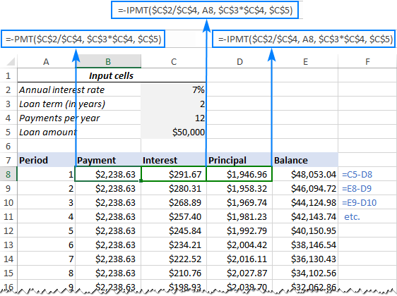
The next thing you do is to create an amortization table with the labels (Period, Payment, Interest, Principal, Balance) in A7:E7. In the Period column, enter a series of numbers equal to the total number of payments (1- 24 in this example):

With all the known components in place, let's get to the most interesting part - loan amortization formulas.
2. Calculate total payment amount (PMT formula)
The payment amount is calculated with the PMT(rate, nper, pv, [fv], [type]) function.
To handle different payment frequencies correctly (such as weekly, monthly, quarterly, etc.), you should be consistent with the values supplied for the rate and nper arguments:
- Rate - divide the annual interest rate by the number of payment periods per year ($C$2/$C$4).
- Nper - multiply the number of years by the number of payment periods per year ($C$3*$C$4).
- For the pv argument, enter the loan amount ($C$5).
- The fv and type arguments can be omitted since their default values work just fine for us (balance after the last payment is supposed to be 0; payments are made at the end of each period).
Putting the above arguments together, we get this formula:
=PMT($C$2/$C$4, $C$3*$C$4, $C$5)
Please pay attention, that we use absolute cell references because this formula should copy to the below cells without any changes.
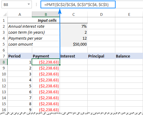
Enter the PMT formula in B8, drag it down the column, and you will see a constant payment amount for all the periods:
3. Calculate interest (IPMT formula)
To find the interest part of each periodic payment, use the IPMT(rate, per, nper, pv, [fv], [type]) function:
=IPMT($C$2/$C$4, A8, $C$3*$C$4, $C$5)
All the arguments are the same as in the PMT formula, except the per argument that specifies the payment period. This argument is supplied as a relative cell reference (A8) because it is supposed to change based on the relative position of a row to which the formula is copied.
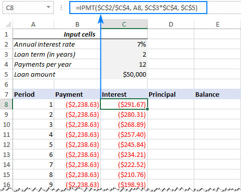
This formula goes to C8, and then you copy it down to as many cells as needed:
4. Find principal (PPMT formula)
To calculate the principal part of each periodic payment, use this PPMT formula:
=PPMT($C$2/$C$4, A8, $C$3*$C$4, $C$5)
The syntax and arguments are exactly the same as in the IPMT formula discussed above:
This formula goes to column D, beginning in D8:
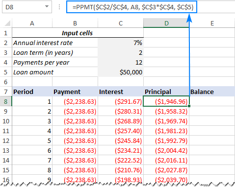
Tip. To check whether your calculations are correct at this point, add up the numbers in the Principal and Interest columns. The sum should be equal to the value in the Payment column in the same row.
5. Get the remaining balance
To calculate the remaining balance for each period, we'll be using two different formulas.
To find the balance after the first payment in E8, add up the loan amount (C5) and the principal of the first period (D8):
=C5+D8
Because the loan amount is a positive number and principal is a negative number, the latter is actually subtracted from the former.
For the second and all succeeding periods, add up the previous balance and this period's principal:
=E8+D9
The above formula goes to E9, and then you copy it down the column. Due to the use of relative cell references, the formula adjusts correctly for each row.
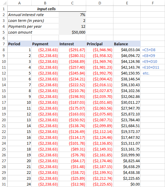
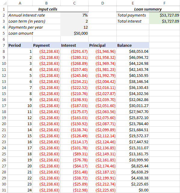
That's it! Our monthly loan amortization schedule is done:
Tip: Return payments as positive numbers
Because a loan is paid out of your bank account, Excel functions return the payment, interest and principal as negative numbers. By default, these values are highlighted in red and enclosed in parentheses as you can see in the image above.
If you prefer to have all the results as positive numbers, put a minus sign before the PMT, IPMT and PPMT functions.
For the Balance formulas, use subtraction instead of addition like shown in the screenshot below:
Amortization schedule for a variable number of periods
In the above example, we built a loan amortization schedule for the predefined number of payment periods. This quick one-time solution works well for a specific loan or mortgage.
If you are looking to create a reusable amortization schedule with a variable number of periods, you will have to take a more comprehensive approach described below.
1. Input the maximum number of periods
In the Period column, insert the maximum number of payments you are going to allow for any loan, say, from 1 to 360. You can leverage Excel's AutoFill feature to enter a series of numbers faster.
2. Use IF statements in amortization formulas
Because you now have many excessive period numbers, you have to somehow limit the calculations to the actual number of payments for a particular loan. This can be done by wrapping each formula into an IF statement. The logical test of the IF statement checks if the period number in the current row is less than or equal to the total number of payments. If the logical test is TRUE, the corresponding function is calculated; if FALSE, an empty string is returned.
Assuming Period 1 is in row 8, enter the following formulas in the corresponding cells, and then copy them across the entire table.
Payment (B8):
=IF(A8<=$C$3*$C$4, PMT($C$2/$C$4, $C$3*$C$4, $C$5), "")
Interest (C8):
=IF(A8<=$C$3*$C$4, IPMT($C$2/$C$4, A8, $C$3*$C$4, $C$5), "")
Principal (D8):
=IF(A8<=$C$3*$C$4,PPMT($C$2/$C$4, A8, $C$3*$C$4, $C$5), "")
Balance:
For Period 1 (E8), the formula is the same as in the previous example:
=C5+D8
For Period 2 (E9) and all subsequent periods, the formula takes this shape:
=IF(A9<=$C$3*$C$4, E8+D9, "")
As the result, you have a correctly calculated amortization schedule and a bunch of empty rows with the period numbers after the loan is paid off.

3. Hide extra periods numbers
If you can live with a bunch of superfluous period numbers displayed after the last payment, you can consider the work done and skip this step. If you strive for perfection, then hide all unused periods by making a conditional formatting rule that sets the font color to white for any rows after the last payment is made.
For this, select all the data rows if your amortization table (A8:E367 in our case) and click Home tab > Conditional formatting > New Rule… > Use a formula to determine which cells to format.
In the corresponding box, enter the below formula that checks if the period number in column A is greater than the total number of payments:
=$A8>$C$3*$C$4
Important note! For the conditional formatting formula to work correctly, be sure to use absolute cell references for the Loan term and Payments per year cells that you multiply ($C$3*$C$4). The product is compared with the Period 1 cell, for which you use a mixed cell reference - absolute column and relative row ($A8).

After that, click the Format… button and pick the white font color. Done!

4. Make a loan summary
To view the summary information about your loan at a glance, add a couple more formulas at the top of your amortization schedule.
Total payments (F2):
=-SUM(B8:B367)
Total interest (F3):
=-SUM(C8:C367)
If you have payments as positive numbers, remove the minus sign from the above formulas.
That's it! Our loan amortization schedule is completed and good to go!
How to make a loan amortization schedule with extra payments in Excel
The amortization schedules discussed in the previous examples are easy to create and follow (hopefully :). However, they leave out a useful feature that many loan payers are interested in - additional payments to pay off a loan faster. In this example, we will look at how to create a loan amortization schedule with extra payments.
1. Define input cells
As usual, begin with setting up the input cells. In this case, let's name these cells like written below to make our formulas easier to read:
- InterestRate - C2 (annual interest rate)
- LoanTerm - C3 (loan term in years)
- PaymentsPerYear - C4 (number of payments per year)
- LoanAmount - C5 (total loan amount)
- ExtraPayment - C6 (extra payment per period)

2. Calculate a scheduled payment
Apart from the input cells, one more predefined cell is required for our further calculations - the scheduled payment amount, i.e. the amount to be paid on a loan if no extra payments are made. This amount is calculated with the following formula:
=IFERROR(-PMT(InterestRate/PaymentsPerYear, LoanTerm*PaymentsPerYear, LoanAmount), "")
Please pay attention that we put a minus sign before the PMT function to have the result as a positive number. To prevent errors in case some of the input cells are empty, we enclose the PMT formula within the IFERROR function.
Enter this formula in some cell (G2 in our case) and name that cell ScheduledPayment.

3. Set up the amortization table
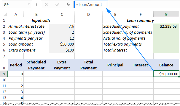
Create a loan amortization table with the headers shown in the screenshot below. In the Period column enter a series of numbers beginning with zero (you can hide the Period 0 row later if needed).
If you aim to create a reusable amortization schedule, enter the maximum possible number of payment periods (0 to 360 in this example).
For Period 0 (row 9 in our case), pull the Balance value, which is equal to the original loan amount. All other cells in this row will remain empty:
Formula in G9:
=LoanAmount
4. Build formulas for amortization schedule with extra payments
This is a key part of our work. Because Excel's built-in functions do not provide for additional payments, we will have to do all the math on our own.
Note. In this example, Period 0 is in row 9 and Period 1 is in row 10. If your amortization table begins in a different row, please be sure to adjust the cell references accordingly.
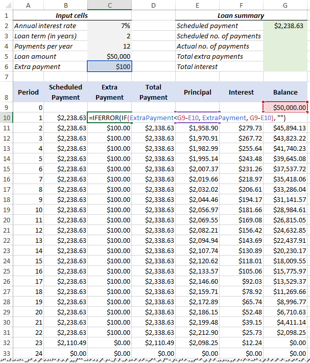
Enter the following formulas in row 10 (Period 1), and then copy them down for all of the remaining periods.
Scheduled Payment (B10):
If the ScheduledPayment amount (named cell G2) is less than or equal to the remaining balance (G9), use the scheduled payment. Otherwise, add the remaining balance and the interest for the previous month.
=IFERROR(IF(ScheduledPayment<=G9, ScheduledPayment, G9+G9*InterestRate/PaymentsPerYear), "")
As an extra precaution, we wrap this and all subsequent formulas in the IFERROR function. This will prevent a bunch of various errors if some of the input cells are empty or contain invalid values.
Extra Payment (C10):
Use an IF formula with the following logic:
If the ExtraPayment amount (named cell C6) is less than the difference between the remaining balance and this period's principal (G9-E10), return ExtraPayment; otherwise use the difference.
=IFERROR(IF(ExtraPayment<G9-E10, ExtraPayment, G9-E10), "")
Tip. If you have variable additional payments, just type the individual amounts directly in the Extra Payment column.
Total Payment (D10)
Simply, add the scheduled payment (B10) and the extra payment (C10) for the current period:
=IFERROR(B10+C10, "")
Principal (E10)
If the schedule payment for a given period is greater than zero, return a smaller of the two values: scheduled payment minus interest (B10-F10) or the remaining balance (G9); otherwise return zero.
=IFERROR(IF(B10>0, MIN(B10-F10, G9), 0), "")
Please note that the principal only includes the part of the scheduled payment (not the extra payment!) that goes toward the loan principal.
Interest (F10)
If the schedule payment for a given period is greater than zero, divide the annual interest rate (named cell C2) by the number of payments per year (named cell C4) and multiply the result by the balance remaining after the previous period; otherwise, return 0.
=IFERROR(IF(B10>0, InterestRate/PaymentsPerYear*G9, 0), "")
Balance (G10)
If the remaining balance (G9) is greater than zero, subtract the principal portion of the payment (E10) and the extra payment (C10) from the balance remaining after the previous period (G9); otherwise return 0.
=IFERROR(IF(G9 >0, G9-E10-C10, 0), "")
Note. Because some of the formulas cross reference each other (not circular reference!), they may display wrong results in the process. So, please do not start troubleshooting until you enter the very last formula in your amortization table.
If all done correctly, your loan amortization schedule at this point should look something like this:
5. Hide extra periods
Set up a conditional formatting rule to hide the values in unused periods as explained in this tip. The difference is that this time we apply the white font color to the rows in which Total Payment (column D) and Balance (column G) are equal to zero or empty:
=AND(OR($D9=0, $D9=""), OR($G9=0, $G9=""))
Voilà, all rows with zero values are hidden from view:

6. Make a loan summary
As a finishing touch of perfection, you can output the most important information about a loan by using these formulas:
Scheduled number of payments:
Multiply the number of years by the number of payments per year:
=LoanTerm*PaymentsPerYear
Actual number of payments:
Count cells in the Total Payment column that are greater than zero, beginning with Period 1:
=COUNTIF(D10:D369,">"&0)
Total extra payments:
Add up cells in the Extra Payment column, beginning with Period 1:
=SUM(C10:C369)
Total interest:
Add up cells in the Interest column, beginning with Period 1:
=SUM(F10:F369)
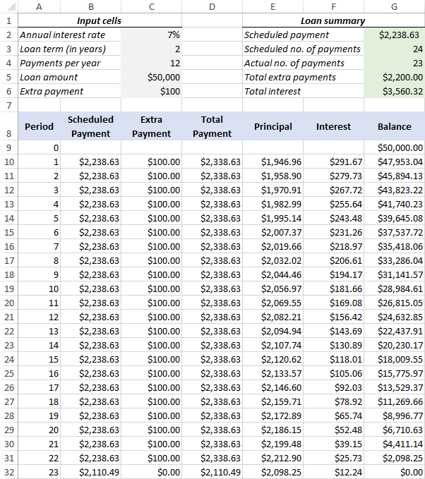
Optionally, hide the Period 0 row, and your loan amortization schedule with additional payments is done! The screenshot below shows the final result:
Amortization schedule Excel template
To make a top-notch loan amortization schedule in no time, make use of Excel's inbuilt templates. Just go to File > New, type "amortization schedule" in the search box and pick the template you like, for example, this one with extra payments:
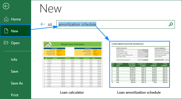
Then save the newly created workbook as an Excel template and reuse whenever you want.
That's how you create a loan or mortgage amortization schedule in Excel. I thank you for reading and hope to see you on our blog next week!
Available downloads
Amortization Schedule examples (.xlsx file)
 by
by
39 comments
I have weekly payments but the date is the same date for the next four payments. How do we get the exact date each week please
Hi! Unfortunately, your question isn't entirely clear. If you're using the payment date as a day of the week, you can add a certain number of days to the initial date, for example, seven days. Read more here: How to add and subtract dates, days, weeks, months and years in Excel. If this is not what you wanted, please explain the problem in more detail.
I'm confused. The point of amortization is for the lender to front load his receipt of interest. To do this, the bulk of the early payments to go interest, and a tiny part goes toward principal paydown. This ratio reverses as you move through the months/years of payments.
Doesn't your chart show the opposite? (With the bulk of the early payments going toward principal, which is wrong in USA lending.)
I just saw that you figured it out yourself in your later comment.
You're overthinking things. The reason the early principal in this example is a lot more than the interest is because the term the 50,000 loan is being paid in is very short compared to the size of the loan. Change the loan amount to be paid for a longer period of time and the principal changes accordingly. The interest caculation is accurate.
I'm trying to create the schedule with extra payments but can't get past steps 1 and 2...
Are we supposed to name the input cells as "InterestRate - C2 (annual interest rate)" or "annual interest rate" in cell A2?
Also, the instruction for step 1 looks like were supposed to type "InterestRate" as a hyperlink somehow in cell D2 but in the example for step 2, that cell is blank.
I have tried the names each way and can't get the balance or schedule payment fields to calculate.
Nevermind... I didn't know about the "Name Box". Now that I know about that, this instruction just got much easier!
Thank you!
Hi Team, these are really nice schedules. However, could you please assist with a schedule that has additional borrowings plus the initial loan.
Initial loan in year 1 and subsequent loans in years 3,4 and 5 respectively.
Thank you Team
Hello!
I am looking for a sheet like this but can hold 30+ vehicles on one sheet and goes vertical with the information and not horizontal. Do you know of anything out there like that?
Hello!
You can change data from vertical to horizontal using the TRANSPOSE function. Here is the article that may be helpful to you: TRANSPOSE function in Excel to change column to row with formula.
I need to add an extra detail of moratorium along with the extra payment feature in the provided sample file. If the file is already provided or created, can you share the same?
Why would the payments not be at the beginning of the period (using type 1 in the excel PMT calculation)? It wouldn’t make sense to make monthly mortgage payments at the end of the month.
Real Estate payments are made in arrears so end of period is appropriate for real estate loans.
Is there a way to keep the Annual Interest Rate cell from rounding up? My actual annual interest rate is 19.6% and when I enter it into the cell, the number is automatically rounded up to 20%, which causes the running balance to be slightly off. I am not very experienced with excel and have probably done something incorrectly. I appreciate your help and information.
Hello!
Here is the article that may be helpful to you: Precision of Excel calculations. Change the cell number format and increase the number of decimal places.
I hope it’ll be helpful.
Am I the only one that is lost here? When setting up the table for extra payments, when i copy the formulas down for the amortization table the boxes the formula references count up as well and start referencing incorrect numbers and in some cases words. How do i copy the formula down the chart but still reference the correct boxes at the top of the table?
Notice how some earlier formulas use $ symbols, such as $C$4. This locks the formula on only ever use the data in C4. Without that, then when you auto fill the formula, it changes itself to C5, C6, C7, etc.
There are some important uses for the shifting cell reference, such as when calculating remaining balance. You want it to use the formula from the previous row, and you want that to keep shifting as it goes down.
I believe there is an error in your loan summary calculations. Although the 30 year loan example has 360 monthly payments, with the FINAL payment in row 367 (because the first 8 rows are header). In other words, you show total payments (F2): =-SUM(B8:B360), but shouldn't it be payments (F2)=-SUM(B8:B367)? And instead of total interest (F3):=-SUM(C8:C360), shouldn't it be total interest (F3):=-SUM(C8:C367)? Also, any chance you could tell me how to modify the spreadsheet for a loan that is interest-only for the first 10 years, then typical Principal & Interest amortization for the final 20 years?
Hi Beth,
Oops, you are absolutely right. Fixed, thank you!
Oops there was an error in my note about the error LOL! I meant to say "Although the 30-year loan example has 360 monthly payments, with the FINAL payment in row 367 (because the first SEVEN rows are header), the totals formulas in F2 and F3 only include up to row 360)". Thanks again. Any help on a loan with interest-only in the beginning, then switching to typical amortization at some point, would be much appreciated.
Thanks for this, I've tried both your template and Microsoft's one to extend beyond 360months. How can I fix this to allow me spread payments to 35years for example?
Ignore my message, I've just used your tutorial to build from scratch. Thanks.
Hi Svetlana,
Thankyou for building this spreadsheet, it's very helpful. I was wondering how I could include a monthly fee into the calculations?
Regards
David
One easy way would be to add it to the Remaining Balance column. In A7 type "Monthly Fee" and then in C7 type in the amount of the fee. For example, if the fee is $25, then type "25" into C7.
Next, add $C$7 to the Balance column.
Doing that will also increase the number of payments. For example, a 30 year mortgage will not be paid off in 30 years with extra fees being thrown onto it, UNLESS those fees are also automatically included in the payment amount. It may be wise to add $C$7 to the Payment column, too.
How do I insert a differnet %rate without changing the existing data? We went from a 15yr fixed 3.125% last November to a 15yr fixed 2.5%. How do I inset that new 2.5% into the table for my next payment? Thanks
I would say simply just add your new interest rate to a cell on top of your spreadsheet and reference it in the next qualifying payment period (formula calculation) instead of the original "Annual interest rate". Call it NewInterestRate and substitute this cell for "AnnualInterestRate" cell.
I believe there is an error in this tutorial (The last payment,)
https://www.ablebits.com/office-addins-blog/create-loan-amortization-schedule-excel/
4. Build formulas for amortization schedule with additional payments
the last total payment cell (D32) is the same as balance in the previous period cell (G31). Interest for that period ($12.24) was not added to (D32). I believe cell (D32) the total payment should be $2110.49 and cell (E32) should be $2098.25.
On the plus side , your tutorial was excellent, much better than other sites.
Thank You.
Hello William,
Thank you for your feedback! From all appearances, you are right. The problem is that I created the amortization schedule with extra payments based on Excel's build-in Loan Amortization Schedule template. In fact, our schedule is a simplified version of Microsoft's one (the goal was to make it more understandable and easier to replicate), and both produce exactly the same results (to make sure of that, just download the loan amortization schedule from your Excel and use it on the same data).
Anyway, we've tried another formula for calculating the total payment and got a different result for the last period ($2110.49 like you mentioned). Just need to do some more testing to make sure in works correctly in other scenarios and work out a plausible explanation why our result is different from Microsoft's :) If all goes well, I will update the formula in the tutorial.
Thank you again for your very thoughtful comment!
I downloaded your payment schedule/ledger with additional payment. The formula is set up to find the monthly interest based on a loan that compounds interest monthly. How do I get this table to show monthly interest based on a loan that compounds the interest annually?
Hi,
Just change the number of payments per year to 1 instead of 12. That should calculate the payment annually (I could be wrong).
Hi,
How do you include a column for variable additional payments? i.e. not necessarily $100 each time.
Thank you
Kira
Hi Kira,
You can just type additional payments directly in the Extra Payment column.
Nice tutorial but what if your totals (e.g. in 1st tip, checking interest + principal payment) do not agree?
How do we handle rounding? Looks to me like the IPMT and PPMT result in rounded results that aren't easy to fix. But further down, where you show extra payments, it appears you're calculating the interest & principal application without use of the IPMT or PPMT functions. Looks to me like the if you want to avoid rounding issues, you should avoid the IPMT & PPMT functions, only use the PMT function to get the periodic payment, and then calculate the periodic amounts with regular arithmetic. Yes? No? Maybe? Thanks
Hi Ken,
In theory, the rounding error cannot exceed 0.5 cents (0.005 dollar). So, the Payment and Interest + Principal may not agree only by 1 cent or less. If the difference is bigger, then there is likely to be something wrong with your model or formulas.
I say "in theory" because in practice, Excel only shows the values rounded to 2 decimal places in cells. The underlying values returned by PMT, IPMT and PPMT are not rounded. To make sure of this, you can choose to show more decimal placed in formula cells.
Dear sir,
Please i need a loan amortization excel sheet that has weekly repayment.
thanks.
Change PaymentsPerYear to 52 and increase the number of rows in your table from 60(?) to 261..
Hi, I am trying to show bi-weekly payments and have it set to 26 payments per year. However, it only shows me the end of month "EOMONTH" dates. How can I change this to show the bi-weekly date?
Hello. Can you please tell me how the following would be calculated?
Add additional funds to each weekly payment (I have weekly payments of 'x' and want to add an extra $60 to each payment.
Add additional lump sum payment once a year
Thank you.