The tutorial shows how to use PMT function in Excel to calculate payments for a loan or investment based on the interest rate, number of payments, and the total loan amount.
Before you borrow money it's good to know how a loan works. Thanks to the Excel financial functions such as RATE, PPMT and IPMT, computing the monthly or any other periodic payment for a loan is easy. In this tutorial, we will have a closer look at the PMT function, discuss its syntax in detail, and show how to build your own PMT calculator in Excel.
What is the PMT function in Excel?
The Excel PMT function is a financial function that calculates the payment for a loan based on a constant interest rate, the number of periods and the loan amount.
"PMT" stands for "payment", hence the function's name.
For example, if you are applying for a two-year car loan with an annual interest rate of 7% and the loan amount of $30,000, a PMT formula can tell you what your monthly payments will be.
For the PMT function to work correctly in your worksheets, please keep in mind these facts:
- To be in line with the general cash flow model, the payment amount is output as a negative number because it's a cash outflow.
- The value returned by the PMT function includes principal and interest but does not include any fees, taxes, or reserve payments that may be associated with a loan.
- A PMT formula in Excel can compute a loan payment for different payment frequencies such as weekly, monthly, quarterly, or annually. This example shows how to do it correctly.
The PMT function is available in Excel for Office 365, Excel 2019, Excel 2016, Excel 2013, Excel 2010 and Excel 2007.
Excel PMT function - syntax and basic uses
The PMT function has the following arguments:
Where:
- Rate (required) - the constant interest rate per period. Can be supplied as percentage or decimal number.
For example, if you make annual payments on a loan at an annual interest rate of 10 percent, use 10% or 0.1 for rate. If you make monthly payments on the same loan, then use 10%/12 or 0.00833 for rate.
- Nper (required) - the number of payments for the loan, i.e. the total number of periods over which the loan should be paid.
For example, if you make annual payments on a 5-year loan, supply 5 for nper. If you make monthly payments on the same loan, then multiply the number of years by 12, and use 5*12 or 60 for nper.
- Pv (required) - the present value, i.e. the total amount that all future payments are worth now. In case of a loan, it's simply the original amount borrowed.
- Fv (optional) - the future value, or the cash balance you wish to have after the last payment is made. If omitted, the future value of the loan is assumed to be zero (0).
- Type (optional) - specifies when the payments are due:
- 0 or omitted - payments are due at the end of each period.
- 1 - payments are due at the beginning of each period.
For example, if you borrow $100,000 for 5 years with an annual interest rate of 7%, the following formula will calculate the annual payment:
=PMT(7%, 5, 100000)
To find the monthly payment for the same loan, use this formula:
=PMT(7%/12, 5*12, 100000)
Or, you can enter the known components of a loan in separate cells and reference those cells in your PMT formula. With the interest rate in B1, no. of years in B2, and loan amount in B3, the formula is as simple as this:
=PMT(B1, B2, B3)
Please remember that the payment is returned as a negative number because this amount will be debited (subtracted) from your bank account.
By default, Excel display the result in the Currency format, rounded to 2 decimal places, highlighted in red and enclosed in parenthesis, as shown in the left part of the image below. The image on the right shows the same result in the General format.

If you'd like to have the payment as a positive number, put a minus sign before either the entire PMT formula or the pv argument (loan amount):
=-PMT(B1, B2, B3)
or
=PMT(B1, B2, -B3)

Tip. To calculate the total amount paid for the loan, multiply the returned PMT value by the number of periods (nper value). In our case, we'd use this equation: 24,389.07*5 and find that the total amount equals $121,945.35.
How to use PMT function in Excel - formula examples
Below you will find a few more examples of an Excel PMT formula that show how to calculate different periodic payments for a car loan, home loan, mortgage loan, and the like.
Full form of PMT function in Excel
For the most part, you can omit the last two arguments in your PMT formulas (like we did in the above examples) because their default values cover the most typical uses cases:
- Fv omitted - implies zero balance after the last payment.
- Type omitted - payments are due at the end of each period.
If your loan conditions are different from the defaults, then use the full form of PMT formula.
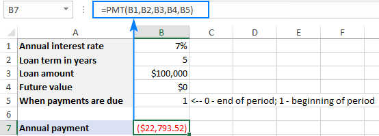
As an example, let's calculate the amount of annual payments based on these input cells:
- B1 - annual interest rate
- B2 - loan term (in years)
- B3 - loan amount
- B4 - future value (balance after the last payment)
- B5 - annuity type:
- 0 (regular annuity) - payments are made at the end of each year.
- 1 (annuity due) - payments are made at the beginning of the period, e.g. rent or lease payments.
Supply these references to your Excel PMT formula:
=PMT(B1, B2, B3, B4, B5)
And you will have this result:

Calculate weekly, monthly, quarterly and semi-annual payments
Depending on the payment frequency, you need to use the following calculations for rate and nper arguments:
- For rate, divide the annual interest rate by the number of payments per year (which is deemed to be equal to the number of compounding periods).
- For nper, multiply the number of years by the number of payments per year.
The below table provides the details:
| Payment Frequency | Rate | Nper |
| Weekly | annual interest rate / 52 | years * 52 |
| Monthly | annual interest rate / 12 | years * 12 |
| Quarterly | annual interest rate / 4 | years * 4 |
| Semi-annual | annual interest rate / 2 | years * 2 |
For instance, to find the amount of a periodic payment on a $5,000 loan with an 8% annual interest rate and a duration of 3 years, use one of the below formulas.
Weekly payment:
=PMT(8%/52, 3*52, 5000)
Monthly payment:
=PMT(8%/12, 3*12, 5000)
Quarterly payment:
=PMT(8%/4, 3*4, 5000)
Semi-annual payment:
=PMT(8%/2, 3*2, 5000)
In all cases, the balance after the last payment is assumed to be $0, and the payments are due at the end of each period.
The screenshot below shows the results of these formulas:

How to make a PMT calculator in Excel
Before you go ahead and borrow money, it stands to reason to compare different loan conditions to find out the options that suit you most. For this, let's create our own Excel loan payment calculator.
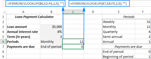
- To begin with, enter the loan amount, interest rate and loan term in separate cells (B3, B4, B5, respectively).
- To be able to choose different periods and specify when the payments are due, create drop-down lists with the following predefined options (B6 and B7):

- Set up the lookup tables for Periods (E2:F6) and Payments are Due (E8:F9) like show in the screenshot below. It is important that text labels in the lookup tables exactly match the items of the corresponding drop-down list.
In the cells next to the drop-down lists, enter the following IFERROR VLOOKUP formulas that will pull the number from the lookup table corresponding to the item selected in the drop-down list.Formula for Periods (C6):
=IFERROR(VLOOKUP(B6, E2:F6, 2, 0), "")Formula for Payments are Due (C7):
=IFERROR(VLOOKUP(B7, E8:F9, 2, 0), "")
- Write a PMT formula to calculate the periodic payment based on your cells. In our case, the formula goes as follows:
=IFERROR(-PMT(B4/C6, B5*C6, B3, 0, C7), "")Please notice the following things:
- The fv argument (0) is hardcoded in the formula because we always want zero balance after the last payment. In case you wish to allow your users to enter any future value, allocate a separate input cell for the fv argument.
- The PMT function is preceded with the minus sign to display the result as a positive number.
- The PMT function is wrapped into IFERROR to hide errors when some input values are not defined.
The above formula goes in B9. And in the neighboring cell (A9) we display a label corresponding to the selected period (B6). For this, simply concatenate the value in B6 and the desired text:
=B6&" Payment"
- Finally, you can hide the lookup tables from view, add a few finishing formatting touches, and your Excel PMT calculator is good to go:

Excel PMT function not working
If your Excel PMT formula is not working or produces wrong results, it's likely to be because of the following reasons:
- A #NUM! error may occur if either the rate argument is a negative number or nper is equal to 0.
- A #VALUE! error occurs if one or more arguments are text values.
- If the result of a PMT formula is much higher or lower than expected, make sure you are consistent with the units supplied for the rate and nper arguments, meaning you have correctly converted the annual interest rate to the period's rate and the number of years to weeks, months, or quarters as shown in this example.
That's how you calculate PMT function in Excel. To have a closer look at the formulas discussed in this tutorial you are welcome to download our sample workbook below. I thank you for reading and hope to see you on our blog next week!
Practice workbook for download
PMT formula in Excel - examples(.xlsx file)
 by
by
2 comments
For example, if you borrow $100,000 for 5 years with an annual interest rate of 7%, the following formula will calculate the annual payment:
=PMT(7%, 5, 100000)
($24,389.07) <-- THIS IS THE ANSWER I GET IN EXCEL
To find the monthly payment for the same loan, use this formula:
=PMT(7%/12, 5*12, 100000)
($1,980.12) <-- THIS IS THE ANSWER I GET IN EXCEL
THESE DO NOT CHECK OUT!
Divide 24,389.07 by 12 = $2,032.42 <-- Does NOT equal the monthly.
Multiply 1,980.12 by 12 = $23,761.44 <-- Does NOT equal the annual.
SOMETHING IS WRONG! Can you please clarify? Thank you.
Hello! This function calculates an annuity payment, where you pay a fixed amount of money for a loan on a regular basis. These amounts cannot and should not be equal! When you repay the loan in installments, you pay less, because the remaining balance of the loan decreases with each payment, and interest depends on it.